莫烦大大TensorFlow学习笔记（9）----可视化

一、Matplotlib【结果可视化】

#import os
#os.environ['TF_CPP_MIN_LOG_LEVEL'] = '2'
import tensorflow as tf
import numpy as np
import matplotlib.pyplot as plt

#添加一个神经层，定义添加神经层的函数
def add_layer(inputs, in_size, out_size, activation_function = None):
    Weights = tf.Variable(tf.random_normal([in_size,out_size]))
    biases = tf.Variable(tf.zeros([1,out_size]) + 0.1)
    Wx_plus_b = tf.matmul(inputs,Weights) + biases #Wx_plus_b代表W*x+b

#如果没有激励函数，即为线性关系，那么直接输出，不需要激励函数（非线性函数）
    if activation_function is None:
        outputs = Wx_plus_b
    else:
        outputs = activation_function(Wx_plus_b) #把这个值传进去
    return outputs
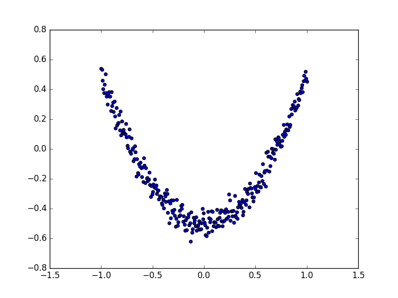
x_data = np.linspace(-1, 1, 300, dtype = np.float32)[:, np.newaxis]
noise = np.random.normal(0, 0.05, x_data.shape).astype(np.float32)
y_data = np.square(x_data) - 0.5 + noise 

xs = tf.placeholder(tf.float32, [None, 1])
ys = tf.placeholder(tf.float32, [None, 1])

l1 = add_layer(xs, 1, 10, activation_function = tf.nn.relu)

#预测值；定义输出层，输入为l1=前一层隐藏层的输出，输入的层数为10=隐藏层神经元的个数，输出的层数为1=输出一般只有1层
prediction = add_layer(l1, 10, 1, activation_function = None)
loss = tf.reduce_mean(tf.reduce_sum(tf.square(ys-prediction),reduction_indices = [1]))
train_step = tf.train.GradientDescentOptimizer(0.1).minimize(loss) #机器要学习的内容，使用优化器提升准确率，学习率为0.1<1，表示以0.1的效率来最小化误差loss

init = tf.global_variables_initializer()

sess = tf.Session() #定义Session，并使用Session来初始化步骤
sess.run(init)

#绘制真实数据
fig = plt.figure() #生成一个画框/画布
ax = fig.add_subplot(1, 1, 1) #将画框分为1行1列，并将图 画在画框的第1个位置
ax.scatter(x_data, y_data) #画散点图
plt.ion() #交互绘制功能，用于连续显示；本次运行时请注释掉这条语句，全局运行不需要注释掉
plt.show() #显示所绘制的图形，但是他只显示当前运行时的图像，不会一直显示多次；在实际运行当中，注释掉上面两条代码，程序才会正常运行，暂时不知道为什么。。。
for i in range(1000): #训练1000次
    sess.run(train_step, feed_dict={xs:x_data, ys:y_data}) #给placeholder喂数据，把x_data赋值给xs
    if i % 50 == 0: #每50步输出一次机器学习的误差
        #print(sess.run(loss, feed_dict={xs:x_data, ys:y_data}))
        #可视化结果与改进
        try:
            ax.lines.remove(lines[0]) #抹去前一条绘制的曲线，在这里我们要先抹去再绘制，防止第一次运行时报错，我们使用try语句
        except Exception:
            pass
        prediction_value = sess.run(prediction, feed_dict={xs:x_data})
        #绘制预测数据
        lines = ax.plot(x_data, prediction_value,'r-',lw=5) #x轴数据，y轴数据，红色的线，线的宽度为5
        plt.pause(0.1) #绘制曲线的时间间隔为0.1秒

二、Tensorboard：【模型可视化】

Tensorboard 可视化好帮手 1

作者: 灰猫 编辑: 莫烦 2016-11-03

学习资料:

• 相关代码
• 为 TF 2017 打造的新版可视化教学代码

注意: 本节内容会用到浏览器, 而且与 tensorboard 兼容的浏览器是 “Google Chrome”. 使用其他的浏览器不保证所有内容都能正常显示.

学会用 Tensorflow 自带的 tensorboard 去可视化我们所建造出来的神经网络是一个很好的学习理解方式. 用最直观的流程图告诉你你的神经网络是长怎样,有助于你发现编程中间的问题和疑问.

效果

好，我们开始吧。

这次我们会介绍如何可视化神经网络。因为很多时候我们都是做好了一个神经网络，但是没有一个图像可以展示给大家看。这一节会介绍一个TensorFlow的可视化工具 — tensorboard :) 通过使用这个工具我们可以很直观的看到整个神经网络的结构、框架。 以前几节的代码为例：相关代码 通过tensorflow的工具大致可以看到，今天要显示的神经网络差不多是这样子的

同时我们也可以展开看每个layer中的一些具体的结构：

好，通过阅读代码和之前的图片我们大概知道了此处是有一个输入层（inputs），一个隐含层（layer），还有一个输出层（output） 现在可以看看如何进行可视化.

搭建图纸

首先从 Input 开始：

# define placeholder for inputs to network

xs = tf.placeholder(tf.float32, [None, 1])

ys = tf.placeholder(tf.float32, [None, 1])

对于input我们进行如下修改： 首先，可以为xs指定名称为x_in:

xs= tf.placeholder(tf.float32, [None, 1],name='x_in')

然后再次对ys指定名称y_in:

ys= tf.placeholder(tf.loat32, [None, 1],name='y_in')

这里指定的名称将来会在可视化的图层inputs中显示出来

使用with tf.name_scope('inputs')可以将xs和ys包含进来，形成一个大的图层，图层的名字就是with tf.name_scope()方法里的参数。

with tf.name_scope('inputs'):

# define placeholder for inputs to network

xs = tf.placeholder(tf.float32, [None, 1])

ys = tf.placeholder(tf.float32, [None, 1])

接下来开始编辑layer ， 请看编辑前的程序片段 ：

def add_layer(inputs, in_size, out_size, activation_function=None):

# add one more layer and return the output of this layer

Weights = tf.Variable(tf.random_normal([in_size, out_size]))

biases = tf.Variable(tf.zeros([1, out_size]) + 0.1)

Wx_plus_b = tf.add(tf.matmul(inputs, Weights), biases)

if activation_function is None:

outputs = Wx_plus_b

else:

outputs = activation_function(Wx_plus_b, )

return outputs

这里的名字应该叫layer, 下面是编辑后的:

def add_layer(inputs, in_size, out_size, activation_function=None):

# add one more layer and return the output of this layer

with tf.name_scope('layer'):

Weights= tf.Variable(tf.random_normal([in_size, out_size]))

# and so on...

在定义完大的框架layer之后，同时也需要定义每一个’框架‘里面的小部件：(Weights biases 和 activation function): 现在现对 Weights 定义： 定义的方法同上，可以使用tf.name.scope()方法，同时也可以在Weights中指定名称W。 即为：

def add_layer(inputs, in_size, out_size, activation_function=None):

#define layer name

with tf.name_scope('layer'):

#define weights name

with tf.name_scope('weights'):

Weights= tf.Variable(tf.random_normal([in_size, out_size]),name='W')

#and so on......

接着继续定义biases ， 定义方式同上。

def add_layer(inputs, in_size, out_size, activation_function=None):

#define layer name

with tf.name_scope('layer'):

#define weights name

with tf.name_scope('weights')

Weights= tf.Variable(tf.random_normal([in_size, out_size]),name='W')

# define biase

with tf.name_scope('Wx_plus_b'):

Wx_plus_b = tf.add(tf.matmul(inputs, Weights), biases)

# and so on....

activation_function 的话，可以暂时忽略。因为当你自己选择用 tensorflow 中的激励函数（activation function）的时候，tensorflow会默认添加名称。 最终，layer形式如下：

def add_layer(inputs, in_size, out_size, activation_function=None):

# add one more layer and return the output of this layer

with tf.name_scope('layer'):

with tf.name_scope('weights'):

Weights = tf.Variable(

tf.random_normal([in_size, out_size]),

name='W')

with tf.name_scope('biases'):

biases = tf.Variable(

tf.zeros([1, out_size]) + 0.1,

name='b')

with tf.name_scope('Wx_plus_b'):

Wx_plus_b = tf.add(

tf.matmul(inputs, Weights),

biases)

if activation_function is None:

outputs = Wx_plus_b

else:

outputs = activation_function(Wx_plus_b, )

return outputs

效果如下：（有没有看见刚才定义layer里面的“内部构件”呢？）

最后编辑loss部分：将with tf.name_scope()添加在loss上方，并为它起名为loss

# the error between prediciton and real data

with tf.name_scope('loss'):

loss = tf.reduce_mean(

tf.reduce_sum(

tf.square(ys - prediction),

eduction_indices=[1]

))

这句话就是“绘制” loss了， 如下：

使用with tf.name_scope()再次对train_step部分进行编辑,如下：

with tf.name_scope('train'):

train_step = tf.train.GradientDescentOptimizer(0.1).minimize(loss)

我们需要使用 tf.summary.FileWriter() (tf.train.SummaryWriter() 这种方式已经在 tf >= 0.12 版本中摒弃) 将上面‘绘画’出的图保存到一个目录中，以方便后期在浏览器中可以浏览。 这个方法中的第二个参数需要使用sess.graph ， 因此我们需要把这句话放在获取session的后面。 这里的graph是将前面定义的框架信息收集起来，然后放在logs/目录下面。

sess = tf.Session() # get session

# tf.train.SummaryWriter soon be deprecated, use following

writer = tf.summary.FileWriter("logs/", sess.graph)

最后在你的terminal（终端）中 ，使用以下命令

tensorboard --logdir logs

同时将终端中输出的网址复制到浏览器中，便可以看到之前定义的视图框架了。

tensorboard 还有很多其他的参数，希望大家可以多多了解, 可以使用 tensorboard --help 查看tensorboard的详细参数 最终的全部代码在这里

可能会遇到的问题

(1) 而且与 tensorboard 兼容的浏览器是 “Google Chrome”. 使用其他的浏览器不保证所有内容都能正常显示.

(2) 同时注意, 如果使用 http://0.0.0.0:6006 网址打不开的朋友们, 请使用 http://localhost:6006, 大多数朋友都是这个问题.

(3) 请确保你的 tensorboard 指令是在你的 logs 文件根目录执行的. 如果在其他目录下, 比如 Desktop 等, 可能不会成功看到图. 比如在下面这个目录, 你要 cd 到 project 这个地方执行 /project > tensorboard --logdir logs

- project

- logs

model.py

env.py

(4) 讨论区的朋友使用 anaconda 下的 python3.5 的虚拟环境, 如果你输入 tensorboard 的指令, 出现报错: "tensorboard" is not recognized as an internal or external command...

解决方法的关键就是需要激活TensorFlow. 管理员模式打开 Anaconda Prompt, 输入 activate tensorflow, 接着按照上面的流程执行 tensorboard 指令.