机器视觉：Convolutional Neural Networks, Receptive Field and Feature Maps

CNN 大概是目前 CV 界最火爆的一款模型了，堪比当年的 SVM。从 2012 年到现在，CNN 已经广泛应用于CV的各个领域，从最初的 classification，到现在的semantic segmentation， object detection，instance segmentation，super resolution 甚至 optical flow 都能看的其身影。还真是，无所不能。

虽然 CNN 的应用可以说是遍地开花，但是细究起来，可以看到 CNN 的基本模型还是万变不离其宗，总是少不了最基础的一些模块，比如 convolution layer, pooling layer 和 fully connected layer，就是基于这些最基础的模块，结合具体的应用，构造了不同的网络结构，进而达到不同的目的。

今天，我们想探讨一下 CNN 网络里面几个基本的概念，掌握并且熟悉这些概念对于理解 CNN 模型有很大的帮助。

我们要理解的概念包括：

• 卷积的基本运算

• receptive field （感受野）

• feature maps

卷积的基本运算

先介绍第一个概念，卷积的运算，我们知道图像处理里面有很多的滤波操作，比如高斯滤波，拉普拉斯滤波，这些其实都是基于卷积的一种运算。

I⊛g" role="presentation">I⊛gI⊛g

这里 I" role="presentation" style="position: relative;">II 表示一张图像，而 g" role="presentation" style="position: relative;">gg 表示卷积核，或者滤波器。卷积简单来说就是对像素邻域的一种操作。这里，我们不讨论卷积的具体表示，我们讨论卷积运算前后图像的尺度变化，这个对于后面理解 receptive field 非常重要。一张 W1×H1" role="presentation" style="position: relative;">W1×H1W1×H1 的图像，经过一个 F×F" role="presentation" style="position: relative;">F×FF×F 卷积核运算，假设卷积运算时候的 stride 为 S" role="presentation" style="position: relative;">SS，那么我们可以求得输出图像的尺寸为：

W2=(W1−F)/S+1H2=(H1−F)/S+1" role="presentation" style="position: relative;">W2=(W1−F)/S+1H2=(H1−F)/S+1W2=(W1−F)/S+1H2=(H1−F)/S+1

比如说，一个 5×5" role="presentation" style="position: relative;">5×55×5 的图像块和一个 3×3" role="presentation" style="position: relative;">3×33×3 的卷积核做卷积，最后输出的图像块的尺寸为 3×3" role="presentation" style="position: relative;">3×33×3，这里我们默认卷积核是逐个像素滑动的，即 stride 为 1，有的时候，我们希望输出图像的尺寸和输入图像的尺寸一样大，这里有不同的处理方式，比较常见的一种方式就是给输入图像的四边补 0，也就是所谓的 zero padding, 我们先把输入图像变大，这样输出图像就会和原来的图像一样大。结合 zero padding，我们可以求得输出图像的大小为：

W2=(W1−F+2P)/S+1H2=(H1−F+2P)/S+1" role="presentation" style="position: relative;">W2=(W1−F+2P)/S+1H2=(H1−F+2P)/S+1W2=(W1−F+2P)/S+1H2=(H1−F+2P)/S+1

Receptive Field

知道了卷积的运算规则，我们来看看 CNN 中的 receptive field 这个概念，receptive field 顾名思义，就是一个像素的感受范围，因为卷积都是基于邻域的操作，所以一般来说，每一层的像素，都是前一层的一个邻域通过卷积运算得到的，我们来看一个层级的 receptive field：

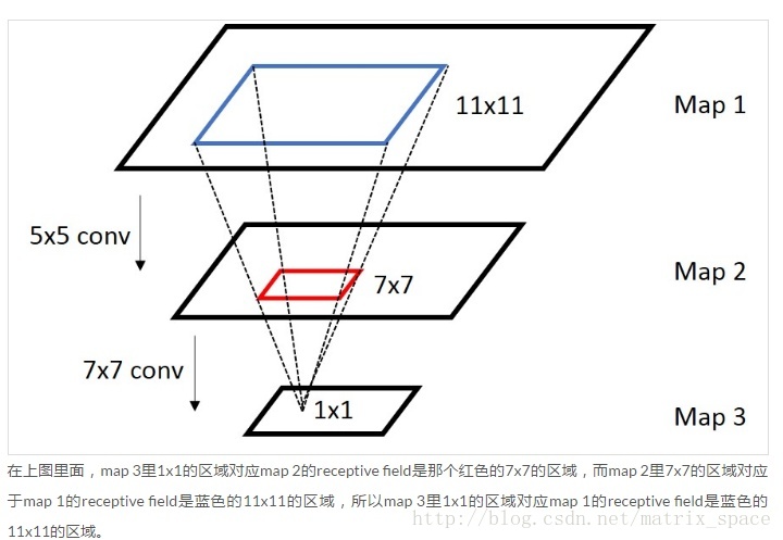
我们看到，最下面一层一个像素，对应的中间一层的 receptive field 是 7×7" role="presentation" style="position: relative;">7×77×7 的一个范围，因为卷积核是 7×7" role="presentation" style="position: relative;">7×77×7，而中间一层的每一个像素，对应最上面一层的 receptive filed 的范围是 5×5" role="presentation" style="position: relative;">5×55×5，那么，最下面一层的每一个像素，对应最上面一层的 receptive field 是多少呢？这里就要用到我们上面介绍的卷积运算的规则，我们可以把上面的卷积规则表示成更一般的表达式：

ri+1=(ri−F+2P)/S+1" role="presentation" style="position: relative;">ri+1=(ri−F+2P)/S+1ri+1=(ri−F+2P)/S+1

ri" role="presentation" style="position: relative;">riri 表示第 i" role="presentation" style="position: relative;">ii 层的 feature map 的尺寸， ri+1" role="presentation" style="position: relative;">ri+1ri+1 表示第 i+1" role="presentation" style="position: relative;">i+1i+1 层的 feature map 的尺寸，那么我们可以反过来求出：

ri=(ri+1−1)×S+F−2P" role="presentation" style="position: relative;">ri=(ri+1−1)×S+F−2Pri=(ri+1−1)×S+F−2P

以上图作为参考，r3=1" role="presentation" style="position: relative;">r3=1r3=1, 这里假设 stride S=1" role="presentation" style="position: relative;">S=1S=1, padding P=0" role="presentation" style="position: relative;">P=0P=0, 第二层到第三层的卷积核是 7×7" role="presentation" style="position: relative;">7×77×7，所以 F=7" role="presentation" style="position: relative;">F=7F=7, 我们可以求得 r2=(1−1)×1+7−2×0=7" role="presentation" style="position: relative;">r2=(1−1)×1+7−2×0=7r2=(1−1)×1+7−2×0=7，所以第二层的 receptive field 是 7×7" role="presentation" style="position: relative;">7×77×7, 那么 r1=(7−1)×1+5−2×0=11" role="presentation" style="position: relative;">r1=(7−1)×1+5−2×0=11r1=(7−1)×1+5−2×0=11，所以第一层的 receptive field是 11×11" role="presentation" style="position: relative;">11×1111×11 所以这就是我们计算每一层 receptive field 的公式，通过层层递推得到。

这是计算不同 layer 之间的 receptive field，有的时候，我们需要计算的是一种坐标映射关系，即 receptive filed 的中心点的坐标，这个坐标映射关系满足下面的关系：

xl=xl+1⋅Sl+1+Fl+1−12−Pl+1" role="presentation">xl=xl+1⋅Sl+1+Fl+1−12−Pl+1xl=xl+1⋅Sl+1+Fl+1−12−Pl+1

在 Fast R-CNN, SPP-Net 等网络中，需要从 feature map 中找到对应的输入图像的 ROI，就是要用上面的表达式从后往前一层一层递推得到：

xL−1=xL⋅SL+FL−12−PLxL−2=xL−1⋅SL−1+FL−1−12−PL−1⋅⋅⋅x1=x2⋅S2+F2−12−P2x0=x1⋅S1+F1−12−P1" role="presentation">xL−1=xL⋅SL+FL−12−PLxL−2=xL−1⋅SL−1+FL−1−12−PL−1⋅⋅⋅x1=x2⋅S2+F2−12−P2x0=x1⋅S1+F1−12−P1xL−1=xL⋅SL+FL−12−PLxL−2=xL−1⋅SL−1+FL−1−12−PL−1⋅⋅⋅x1=x2⋅S2+F2−12−P2x0=x1⋅S1+F1−12−P1

从上面可以看到，如果我们知道第 L" role="presentation" style="position: relative;">LL 层中一个像素点的位置 xL" role="presentation" style="position: relative;">xLxL，我们可以计算出输入图像上对应的 receptive filed 的中心点的位置 x0" role="presentation" style="position: relative;">x0x0, 这个最后可以总结成如下的表达式：

x0=gL(xL)=αL(xL−1)+βLαL=∏l=1LSlβL=1+∑l=1L(∏k=1l−1Sk)(Fk−12−Pk)" role="presentation">x0=gL(xL)=αL(xL−1)+βLαL=∏l=1LSlβL=1+∑l=1L(∏k=1l−1Sk)(Fk−12−Pk)x0=gL(xL)=αL(xL−1)+βLαL=∏l=1LSlβL=1+∑l=1L(∏k=1l−1Sk)(Fk−12−Pk)

SPP-net 中，把 feature map 中的一个区域，映射到输入图像上的 ROI 的时候，做了一些处理，就是让每一层的 padding 都等于卷积核的半径，这样坐标最后只和 stride 有关。

Feature map

最后，我们说一下 feature map，这个可以说是 CNN 和传统的 MLP 的最大的不同，Feature map 中的神经元是共享权重系数的，feature map 中的每一个神经元对应的就是前一层的 feature map 中的某个邻域，反应的是这个邻域与卷积核做卷积之后的一种响应，因为这是一种局部的响应，所以 feature map 可以记录 feature ，也可以记录 location，响应的位置，利用这个特性，可以用来做 目标检测。

参考：

https://zhuanlan.zhihu.com/p/24780433 晓雷机器学习笔记

http://cs231n.stanford.edu/ CS231n: Convolutional Neural Networks for Visual Recognition

iccv2015_tutorial_convolutional_feature_maps_kaiminghe