ProE常用曲线方程：Python Matplotlib 版本代码（蝴蝶曲线）

花纹的生成可以使用贴图的方式，同样也可以使用方程，本文列出了几种常用曲线的方程式，以取代贴图方式完成特定花纹的生成。

注意极坐标的使用.................

前面部分基础资料，参考：Python：Matplotlib 画曲线和柱状图（Code）

Pyplot教程：https://matplotlib.org/gallery/index.html#pyplots-examples

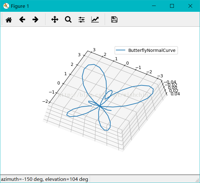
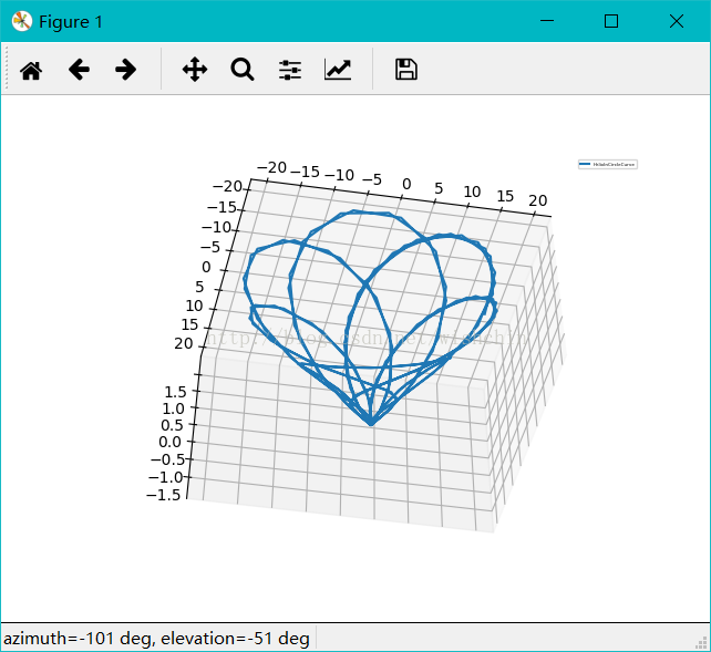
顾名思义，蝴蝶曲线（Butterfly curve ）就是曲线形状如同蝴蝶。蝴蝶曲线如图所示，以方程描述，是一条六次平面曲线。如果大家觉得这个太过简单，别着急，还有第二种。如图所示，以方程描述，这是一个极坐标方程。通过改变这个方程中的变量θ，可以得到不同形状与方向的蝴蝶曲线。如果再施以复杂的组合和变换，我们看到的就完全称得上是一幅艺术品了。

Python代码：

import numpy as np
import matplotlib.pyplot as plt
import os,sys,caffe

import matplotlib as mpl
from mpl_toolkits.mplot3d import Axes3D  #draw lorenz attractor
# %matplotlib inline
from math import sin, cos, pi
import math

def mainex():
    #drawSpringCrurve();#画柱坐标系螺旋曲线
    #HelicalCurve();#采用柱坐标系#尖螺旋曲线
    #Votex3D();
    #phoenixCurve();
    #ButterflyCurve();
    #ButterflyNormalCurve();
    #dicareCurve2d();
    #WindmillCurve3d();
    #HelixBallCurve();#球面螺旋线
    #AppleCurve();
    #HelixInCircleCurve();#使用scatter，排序有问题
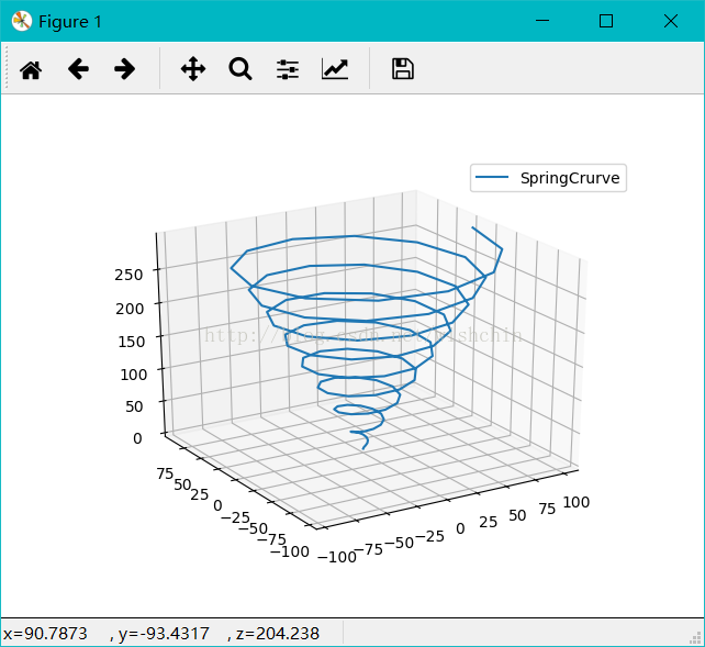
    seperialHelix();

def drawSpringCrurve():
    #碟形弹簧
    #圓柱坐标
    #方程：
    #import matplotlib as mpl
    #from mpl_toolkits.mplot3d import Axes3D
    #import numpy as np
    #import matplotlib.pyplot as plt
    mpl.rcParams['legend.fontsize'] = 10;

    fig = plt.figure();
    ax = fig.gca(projection='3d');

    # Prepare arrays x, y, z
    #theta = np.linspace(-4 * np.pi, 4 * np.pi, 100)
    #z = np.linspace(-2, 2, 100)
    #r = z**2 + 1

    t = np.arange(0,100,1);
    r = t*0 +20;
    theta = t*3600 ;

    z = np.arange(0,100,1);
    for i in range(100):
        z[i] =(sin(3.5*theta[i]-90))+24*t[i];

    x = r * np.sin(theta);
    y = r * np.cos(theta);

    ax.plot(x, y, z, label='SpringCrurve');
    ax.legend();

    plt.show();

def HelicalCurve():
    #螺旋曲线#采用柱坐标系
    t = np.arange(0,100,1);
    r =t ;
    theta=10+t*(20*360);
    z =t*3;

    x = r * np.sin(theta);
    y = r * np.cos(theta);

    mpl.rcParams['legend.fontsize'] = 10;
    fig = plt.figure();
    ax = fig.gca(projection='3d');

    ax.plot(x, y, z, label='HelicalCurve');
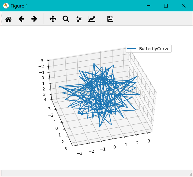
    ax.legend();

    plt.show();

def ButterflyCurve():
    #蝶形曲线，使用球坐标系#或许公式是错误的，应该有更加复杂的公式
    t = np.arange(0,4,0.01);

    r = 8 * t;
    theta = 3.6 * t * 2*1 ;
    phi   = -3.6 * t * 4*1;

    x = t*1;
    y = t*1;
    #z = t*1;
    z =0
    for i in range(len(t)):
        x[i] = r[i] * np.sin(theta[i])*np.cos(phi[i]);
        y[i] = r[i] * np.sin(theta[i])*np.sin(phi[i]);
        #z[i] = r[i] * np.cos(theta[i]);
    mpl.rcParams['legend.fontsize'] = 10;
    fig = plt.figure();
    ax = fig.gca(projection='3d');

    ax.plot(x, y, z, label='ButterflyCurve');
    #ax.scatter(x, y, z, label='ButterflyCurve');
    ax.legend();

    plt.show();

def ButterflyNormalCurve():
    #蝶形曲线，使用球坐标系#或许公式是错误的，应该有更加复杂的公式
    #螺旋曲线#采用柱坐标系
    #t = np.arange(0,100,1);

    theta=np.arange(0,6,0.1);#(0,72,0.1);
    r =theta*0;
    z =theta*0;

    x =theta*0;
    y =theta*0;
    for i in range(len(theta)):
        r[i] = np.power(math.e,sin(theta[i]))- 2*cos(4*theta[i])
        + np.power( sin(1/24 * (2*theta[i] -pi ) ) , 5 );
        #x[i] = r[i] * np.sin(theta[i]);
        #y[i] = r[i] * np.cos(theta[i]);
    x = r * np.sin(theta);
    y = r * np.cos(theta);
    mpl.rcParams['legend.fontsize'] = 10;
    fig = plt.figure();
    ax = fig.gca(projection='3d');

    ax.plot(x, y, z, label='ButterflyNormalCurve');
    ax.legend();

    plt.show();

def phoenixCurve():
    #蝶形曲线，使用球坐标系
    t = np.arange(0,100,1);

    r = 8 * t;
    theta = 360 * t * 4 ;
    phi   = -360 * t * 8;

    x = t*1;
    y = t*1;
    z = t*1;
    for i in range(len(t)):
        x[i] = r[i] * np.sin(theta[i])*np.cos(phi[i]);
        y[i] = r[i] * np.sin(theta[i])*np.sin(phi[i]);
        z[i] = r[i] * np.cos(theta[i]);
    mpl.rcParams['legend.fontsize'] = 10;
    fig = plt.figure();
    ax = fig.gca(projection='3d');

    ax.plot(x, y, z, label='phoenixCurve');
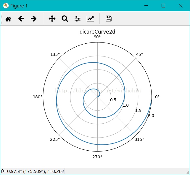
    ax.legend();

    plt.show();

def dicareCurve2d():

    r = np.arange(0, 2, 0.01)
    theta = 2 * np.pi * r

    ax = plt.subplot(111, projection='polar')
    ax.plot(theta, r)
    ax.set_rmax(2)
    ax.set_rticks([0.5, 1, 1.5, 2])  # Less radial ticks
    ax.set_rlabel_position(-22.5)  # Move radial labels away from plotted line
    ax.grid(True)

    ax.set_title("dicareCurve2d", va='bottom')
    plt.show();

def WindmillCurve3d():
    #风车曲线
    t = np.arange(0,2,0.01);
    r =t*0+1 ;

    #r=1
    ang =36*t;#ang =360*t;
    s =2*pi*r*t;

    x = t*1;
    y = t*1;
    for i in range(len(t)):
        x[i] = s[i]*cos(ang[i]) +s[i]*sin(ang[i]) ;
        y[i] = s[i]*sin(ang[i]) -s[i]*cos(ang[i]) ;

    z =t*0;

    mpl.rcParams['legend.fontsize'] = 10;
    fig = plt.figure();
    ax = fig.gca(projection='3d');

    ax.plot(x, y, z, label='WindmillCurve3d');
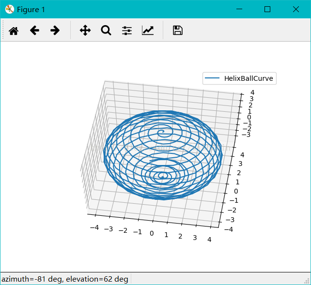
    ax.legend();

    plt.show();

def HelixBallCurve():
    #螺旋曲线，使用球坐标系
    t = np.arange(0,2,0.005);
    r =t*0+4 ;
    theta =t*1.8
    phi =t*3.6*20

    x = t*1;
    y = t*1;
    z = t*1;
    for i in range(len(t)):
        x[i] = r[i] * np.sin(theta[i])*np.cos(phi[i]);
        y[i] = r[i] * np.sin(theta[i])*np.sin(phi[i]);
        z[i] = r[i] * np.cos(theta[i]);
    mpl.rcParams['legend.fontsize'] = 10;
    fig = plt.figure();
    ax = fig.gca(projection='3d');

    ax.plot(x, y, z, label='HelixBallCurve');
    ax.legend();

    plt.show();

def seperialHelix():
    #螺旋曲线，使用球坐标系
    t = np.arange(0,2,0.1);
    n = np.arange(0,2,0.1);
    r =t*0+4 ;
    theta =n*1.8 ;
    phi =n*3.6*20;

    x = t*0;
    y = t*0;
    z = t*0;
    for i in range(len(t)):
        x[i] = r[i] * np.sin(theta[i])*np.cos(phi[i]);
        y[i] = r[i] * np.sin(theta[i])*np.sin(phi[i]);
        z[i] = r[i] * np.cos(theta[i]);

    mpl.rcParams['legend.fontsize'] = 10;
    fig = plt.figure();
    ax = fig.gca(projection='3d');

    ax.plot(x, y, z, label='ButterflyCurve');
    ax.legend();

    plt.show();

def AppleCurve():
    #螺旋曲线
    t = np.arange(0,2,0.01);

    l=2.5
    b=2.5
    x =  t*1;
    y =  t*1;
    z =0;#z=t*0;
    n = 36
    for i in range(len(t)):
        x[i]=3*b*cos(t[i]*n)+l*cos(3*t[i]*n)
        y[i]=3*b*sin(t[i]*n)+l*sin(3*t[i]*n)

    #x = r * np.sin(theta);
    #y = r * np.cos(theta);

    mpl.rcParams['legend.fontsize'] = 10;
    fig = plt.figure();
    ax = fig.gca(projection='3d');

    ax.plot(x, y, z, label='AppleCurve');
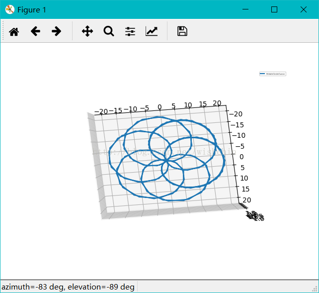
    ax.legend();

    plt.show();

def HelixInCircleCurve():
    #园内螺旋曲线#采用柱坐标系
    t = np.arange(-1,1,0.01);

    theta=t*36 ;#360 deta 0.005鸟巢网 #36 deta 0.005 圆内曲线
    x =  t*1;
    y =  t*1;
    z =  t*1;
    r =  t*1;
    n = 1.2
    for i in range(len(t)):
        r[i]=10+10*sin(n*theta[i]);
        z[i]=2*sin(n*theta[i]);
        x[i] = r[i] * np.sin(theta[i]);
        y[i] = r[i] * np.cos(theta[i]);

    mpl.rcParams['legend.fontsize'] = 3;
    fig = plt.figure();
    ax = fig.gca(projection='3d');

    ax.plot(x, y, z, label='HelixInCircleCurve');
    #ax.scatter(x, y, z, label='HelixInCircleCurve');
    ax.legend();

    plt.show();

def Votex3D():

    def midpoints(x):
        sl = ()
        for i in range(x.ndim):
            x = (x[sl + np.index_exp[:-1]] + x[sl + np.index_exp[1:]]) / 2.0
            sl += np.index_exp[:]
        return x

    # prepare some coordinates, and attach rgb values to each
    r, g, b = np.indices((17, 17, 17)) / 16.0
    rc = midpoints(r)
    gc = midpoints(g)
    bc = midpoints(b)

    # define a sphere about [0.5, 0.5, 0.5]
    sphere = (rc - 0.5)**2 + (gc - 0.5)**2 + (bc - 0.5)**2 < 0.5**2

    # combine the color components
    colors = np.zeros(sphere.shape + (3,))
    colors[..., 0] = rc
    colors[..., 1] = gc
    colors[..., 2] = bc

    # and plot everything
    fig = plt.figure();
    ax = fig.gca(projection='3d');
    ax.voxels(r, g, b, sphere,
              facecolors=colors,
              edgecolors=np.clip(2*colors - 0.5, 0, 1),  # brighter
              linewidth=0.5);
    ax.set(xlabel='r', ylabel='g', zlabel='b');
    plt.show();

def drawFiveFlower():
    theta=np.arange(0,2*np.pi,0.02)
    #plt.subplot(121,polar=True)
    #plt.plot(theta,2*np.ones_like(theta),lw=2)
    #plt.plot(theta,theta/6,'--',lw=2)
    #plt.subplot(122,polar=True)
    plt.subplot(111,polar=True)
    plt.plot(theta,np.cos(5*theta),'--',lw=2)
    plt.plot(theta,2*np.cos(4*theta),lw=2)
    plt.rgrids(np.arange(0.5,2,0.5),angle=45)
    plt.thetagrids([0,45,90]);

    plt.show(); 

if __name__ == '__main__':
    import argparse
    mainex();

画图结果：