[Scikit-learn] 2.1 Clustering - Variational Bayesian Gaussian Mixture

最重要的一点是：Bayesian GMM为什么拟合的更好？

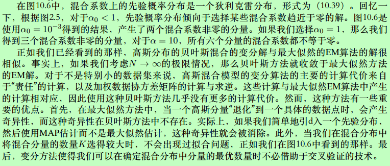
PRML 这段文字做了解释：

Ref: http://freemind.pluskid.org/machine-learning/deciding-the-number-of-clusterings/

链接中提到了一些其他的无监督聚类。

From: http://scikit-learn.org/stable/modules/mixture.html#variational-bayesian-gaussian-mixture

Due to its Bayesian nature, the variational algorithm needs more hyper- parameters than expectation-maximization,

the most important of these being the concentration parameter weight_concentration_prior.

• Specifying a low value for the concentration prior will make the model put most of the weight on few components set the remaining components weights very close to zero.
• High values of the concentration prior will allow a larger number of components to be active in the mixture.

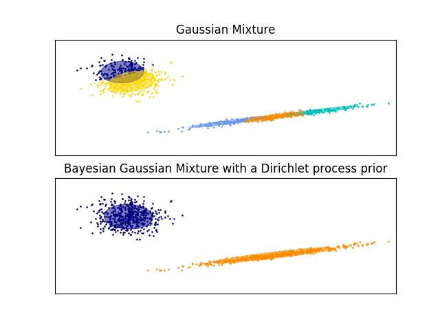
The examples below compare Gaussian mixture models with a fixed number of components, to the variational Gaussian mixture models with a Dirichlet process prior. Here, a classical Gaussian mixture is fitted with 5 components on a dataset composed of 2 clusters.

We can see that the variational Gaussian mixture with a Dirichlet process prior is able to limit itself to only 2 components whereas the Gaussian mixture fits the data with a fixed number of components that has to be set a priori by the user. In this case the user has selected n_components=5 which does not match the true generative distribution of this toy dataset. Note that with very little observations, the variational Gaussian mixture models with a Dirichlet process prior can take a conservative stand, and fit only one component.

Dirichlet distribution 具有自动的特征选取的作用，找出起主要作用的components。

5 for GMM
[ 0.1258077   0.23638361  0.23330578  0.26361639  0.14088652]
5 for Bayesian GMM
[ 0.001019    0.00101796  0.49948856  0.47955123  0.01892325]

问题来了：

为什么dirichlet会让三个的权重偏小，而GMM却没有，难道是收敛速度不同？

应该跟速度没有关系。加了先验后，后验变为了dirichlet，那么参数的估计过程中便具备了dirichlet的良好性质。

原始数据

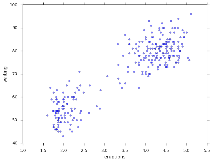
Our data set will be the classic Old Faithful dataset.

plt.scatter(data['eruptions'], data['waiting'], alpha=0.5);
plt.xlabel('eruptions');
plt.ylabel('waiting');

如何拟合？

from sklearn.mixture import BayesianGaussianMixture

mixture_model = BayesianGaussianMixture(
    n_components=10,
    random_state=5,  # control the pseudo-random initialization
    weight_concentration_prior_type='dirichlet_distribution',
    weight_concentration_prior=1.0,  # parameter of the Dirichlet component prior
    max_iter=200,  # choose this to be big in case it takes a long time to fit
)
mixture_model.fit(data);

Ref: http://scikit-learn.org/stable/auto_examples/mixture/plot_concentration_prior.html

可直接调用该程式：

plot_ellipses(ax1, model.weights_, model.means_, model.covariances_)

def plot_ellipses(ax, weights, means, covars):
    """
    Given a list of mixture component weights, means, and covariances,
    plot ellipses to show the orientation and scale of the Gaussian mixture dispersal.
    """
    for n in range(means.shape[0]):
        eig_vals, eig_vecs = (covars[n])
        unit_eig_vec = eig_vecs[0] / np.linalg.norm(eig_vecs[0])
        angle = np.arctan2(unit_eig_vec[1], unit_eig_vec[0])
        # Ellipse needs degrees
        angle = 180 * angle / np.pi
        # eigenvector normalization
        eig_vals = 2 * np.sqrt(2) * np.sqrt(eig_vals)
        ell = mpl.patches.Ellipse(
            means[n], eig_vals[0], eig_vals[1],
            180 + angle,
            edgecolor=None,)
        ell2 = mpl.patches.Ellipse(
            means[n], eig_vals[0], eig_vals[1],
            180 + angle,
            edgecolor='black',
            fill=False,
            linewidth=1,)
        ell.set_clip_box(ax.bbox)
        ell2.set_clip_box(ax.bbox)
        ell.set_alpha(weights[n])
        ell.set_facecolor('#56B4E9')
        ax.add_artist(ell)
        ax.add_artist(ell2)

plot_results(
    mixture_model,
    data['eruptions'], data['waiting'],
    'weight_concentration_prior={}'.format(1.0))

def plot_results(model, x, y, title, plot_title=False):

    fig, ax = plt.subplots(3, 1, sharex=False)
    # 上面是ax没用，以下重新定义了ax1 ax2
    gs = gridspec.GridSpec(3, 1)　　# 自定义子图位置
    ax1 = plt.subplot(gs[0:2, 0])
    # 以下四行是固定套路
    ax1.set_title(title)
    ax1.scatter(x, y, s=5, marker='o', alpha=0.8)
    ax1.set_xticks(())
    ax1.set_yticks(())
    n_components = model.get_params()['n_components']

    plot_ellipses(ax1, model.weights_, model.means_, model.covariances_)

    # ax1:画椭圆
    # ax2:画权重
    ax2 = plt.subplot(gs[2, 0])
    ax2.get_xaxis().set_tick_params(direction='out')
    ax2.yaxis.grid(True, alpha=0.7)
    for k, w in enumerate(model.weights_):
        ax2.bar(k, w, width=0.9, color='#56B4E9', zorder=3,
                align='center', edgecolor='black')
        ax2.text(k, w + 0.007, "%.1f%%" % (w * 100.),
                 horizontalalignment='center')
    ax2.set_xlim(-.6, n_components - .4)
    ax2.set_ylim(0., 1.1)
    ax2.tick_params(axis='y', which='both', left='off',
                    right='off', labelleft='off')
    ax2.tick_params(axis='x', which='both', top='off')

    if plot_title:
        ax1.set_ylabel('Estimated Mixtures')
        ax2.set_ylabel('Weight of each component')

查看拟合过程：

lower_bounds = []
mixture_model = BayesianGaussianMixture(
    n_components    =10,
    covariance_type ='full',
    max_iter        =1,
    random_state    =2,
    weight_concentration_prior_type ='dirichlet_distribution',
    warm_start      =True,
)
# 设置model.fit为只递归一次
for i in range(200):
    mixture_model.fit(data)
    if mixture_model.converged_: break
    lower_bounds.append(mixture_model.lower_bound_)
    if i%5==0 and i<60:
        plt.figure();
        plot_results(
            mixture_model,
            data['eruptions'], data['waiting'],
            'EM step={}, lower_bound={}'.format(
                i, mixture_model.lower_bound_)
        );

plt.figure();
plt.plot(lower_bounds);
plt.gca().set_xlabel('step')
plt.gca().set_ylabel('lower bound')

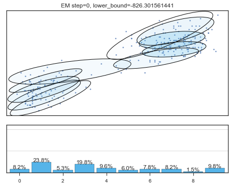
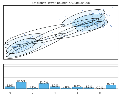
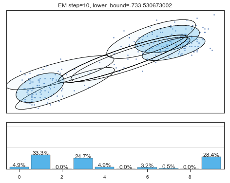
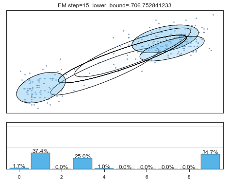
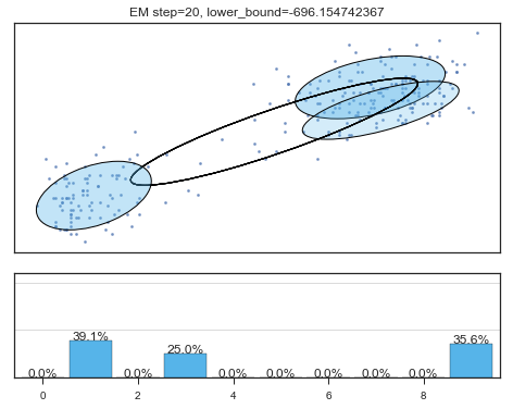
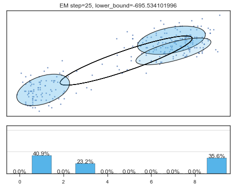
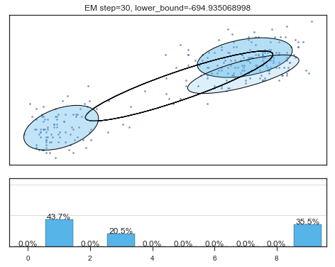
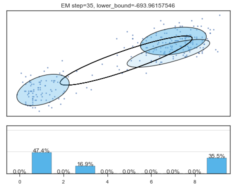
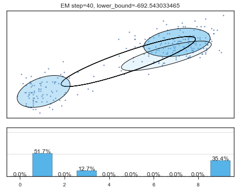
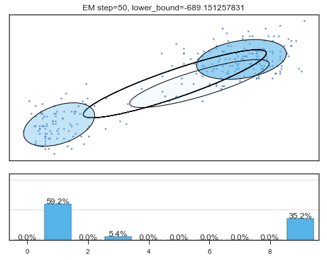
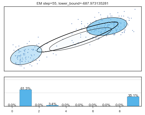
Lower bound 逐渐增加。

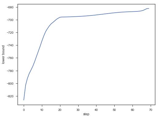
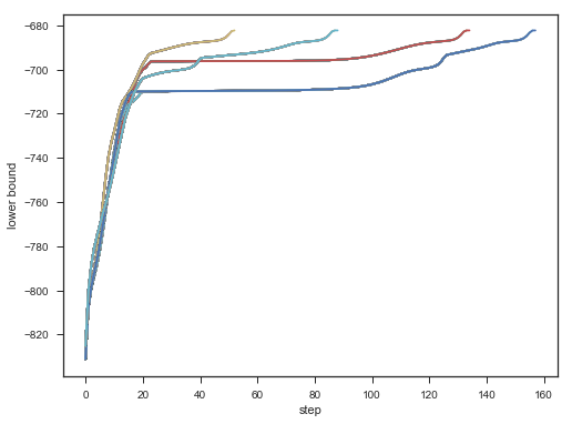
不同初始，效果对比：

for seed in range(6,11):
    lower_bounds = []
    mixture_model = BayesianGaussianMixture(
        n_components=10,
        covariance_type='full',
        max_iter=1,
        random_state=seed,
        weight_concentration_prior_type='dirichlet_distribution',
        warm_start=True,
    )
    for i in range(200):
        mixture_model.fit(data)
        if mixture_model.converged_: break
        lower_bounds.append(mixture_model.lower_bound_)
        plt.plot(lower_bounds);
plt.gca().set_xlabel('step')
plt.gca().set_ylabel('lower bound');

Result: