深度学习基础 Probabilistic Graphical Models | Statistical and Algorithmic Foundations of Deep Learning

目录

• Probabilistic Graphical Models
  • Statistical and Algorithmic Foundations of Deep Learning
  • 01 An overview of DL components
    • Historical remarks: early days of neural networks
    • Reverse-mode automatic differentiation (aka backpropagation)
    • Modern building blocks: units, layers, activations functions, loss functions, etc.
  • 02 Similarities and differences between GMs and NNs
    • Graphical models vs. computational graphs
    • Sigmoid Belief Networks as graphical models
    • Deep Belief Networks and Boltzmann Machines
  • 03 Combining DL methods and GMs
    • Using outputs of NNs as inputs to GMs
    • GMs with potential functions represented by NNs q NNs with structured outputs
      • Contextual Explanation Networks (CENs)
  • 04 Bayesian Learning of NNs
    • Bayesian learning of NN parameters q Deep kernel learning

原文链接：小样本学习与智能前沿

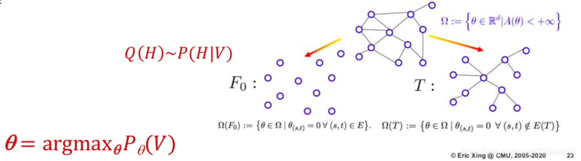
Probabilistic Graphical Models

Statistical and Algorithmic Foundations of Deep Learning

Author: Eric Xing

01 An overview of DL components

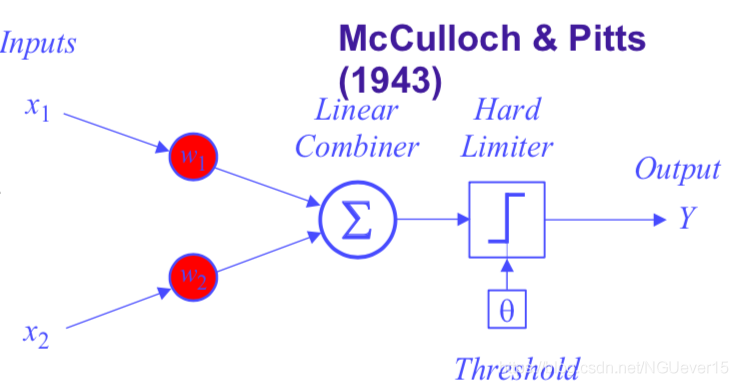
Historical remarks: early days of neural networks

我们知道生物神经元是这样的：



上游细胞通过轴突（Axon）将神经递质传送给下游细胞的树突。 人工智能受到该原理的启发，是按照下图来构造人工神经元（或者是感知器）的。



类似的，生物神经网络 —— > 人工神经网络


Reverse-mode automatic differentiation (aka backpropagation)

下面我们来看看具体的感知器学习算法。



假设这是一个回归问题x->y，\(y = f(x)+\eta\)$, 则目标函数为



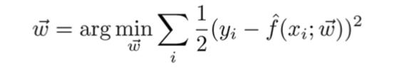
为了求出该函数的解，我们需要对其求导，具体的：



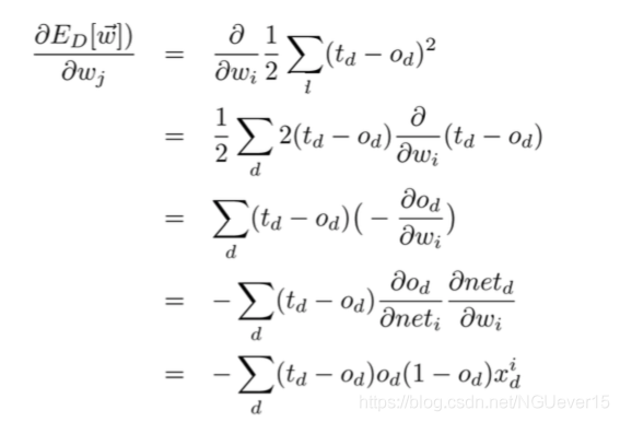
其中

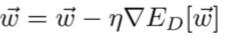
由此\(w\)的更新公式为：

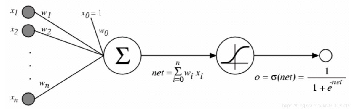
下面我们来说说神经网络模型：



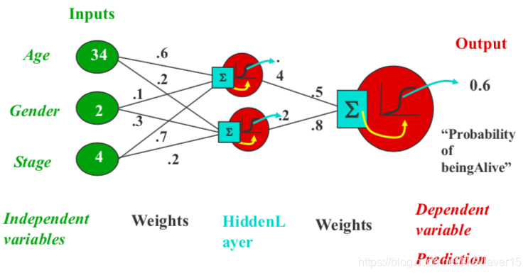
其中，隐藏单元没有目标。

人工神经网络不过是可以由计算图表示的复杂功能组成。



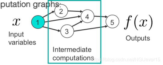
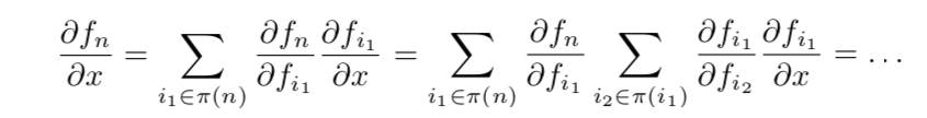
通过应用链式规则并使用反向累积，我们得到：



该算法通常称为反向传播。 如果某些功能是随机的怎么办？使用随机反向传播！现代软件包可以自动执行此操作（稍后再介绍）

Modern building blocks: units, layers, activations functions, loss functions, etc.

常用激活函数：

• Linear and ReLU
• Sigmoid and tanh
• Etc.

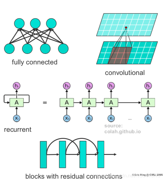
网络层：

• Fully connected
• Convolutional & pooling
• Recurrent
• ResNets
• Etc.
  
  -
  
  

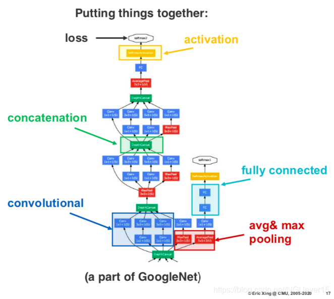
也就是说基本构成要素的可以任意组合，如果有多种损失功能的话，可以实现多目标预测和转移学习等。 只要有足够的数据，更深的架构就会不断改进。

Feature learning

成功学习中间表示[Lee et al ICML 2009，Lee et al NIPS 2009]



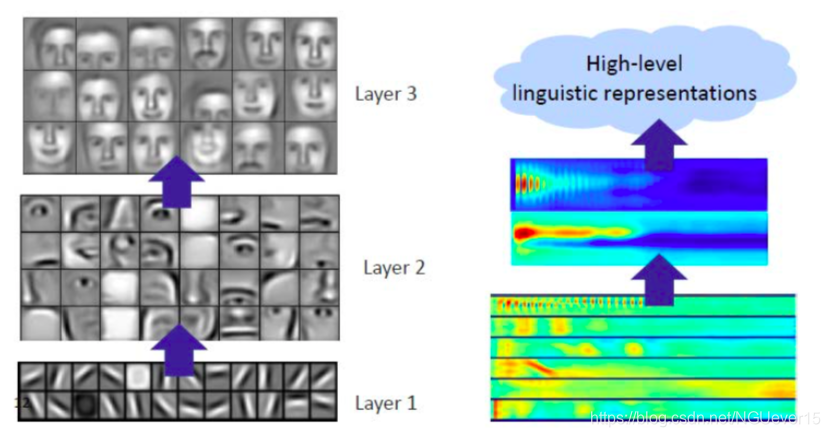
表示学习：网络学习越来越多的抽象数据表示形式，这些数据被“解开”，即可以进行线性分离。

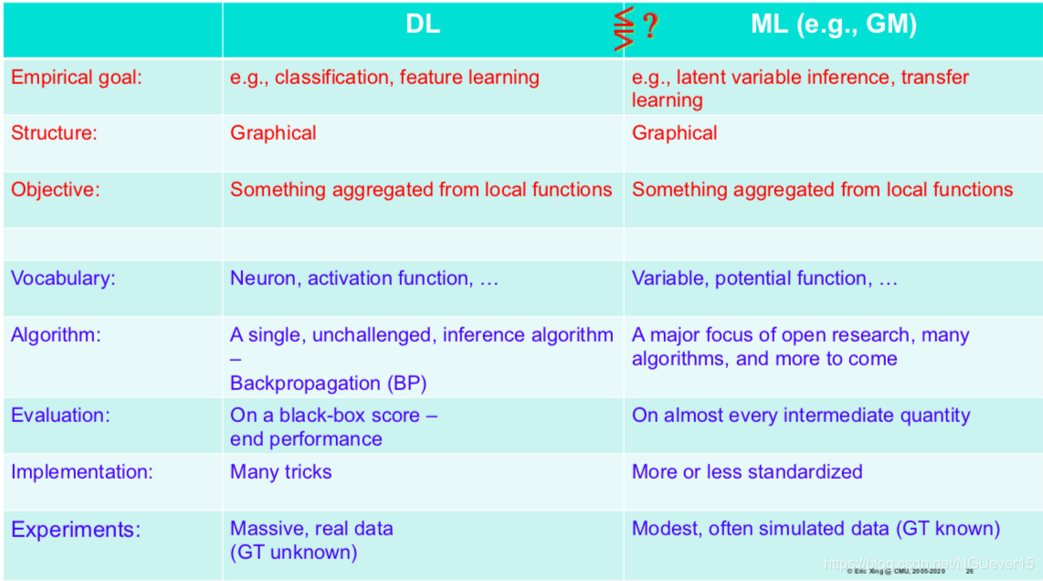
02 Similarities and differences between GMs and NNs

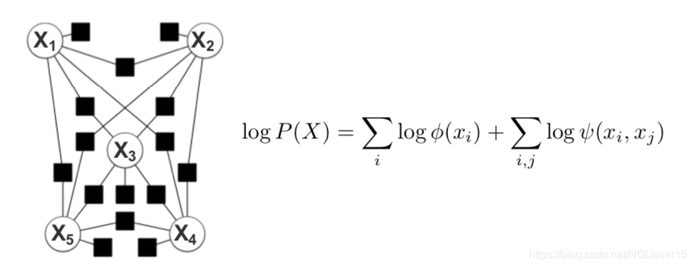
Graphical models vs. computational graphs

Graphical models:

• 用于以图形形式编码有意义的知识和相关的不确定性的表示形式
• 学习和推理基于经过充分研究（依赖于结构）的技术（例如EM，消息传递，VI，MCMC等）的丰富工具箱
• 图形代表模型
  
  
  
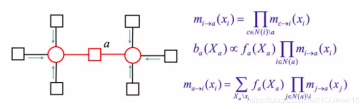
  Utility of the graph
• 一种用于从局部结构综合全局损失函数的工具(潜在功能，特征功能等)
• 一种设计合理有效的推理算法的工具(总和，均值场等)
• 激发近似和惩罚的工具(结构化MF，树近似等)
• 用于监视理论和经验行为以及推理准确性的工具

Utility of the loss function

• 学习算法和模型质量的主要衡量指标

Deep neural networks :

• 学习有助于最终指标上的计算和性能的表示形式（中间表示形式不保证一定有意义）
• 学习主要基于梯度下降法（aka反向传播）；推论通常是微不足道的，并通过“向前传递”完成
• 图形代表计算

Utility of the network

• 概念上综合复杂决策假设的工具（分阶段的投影和聚合）
• 用于组织计算操作的工具（潜在状态的分阶段更新）
• 用于设计加工步骤和计算模块的工具（逐层并行化）
• 在评估DL推理算法方面没有明显的用途

到目前为止，图形模型是概率分布的表示，而神经网络是函数近似器（无概率含义）。有些神经网络实际上是图形模型（即单位/神经元代表随机变量）：

• 玻尔兹曼机器Boltzmann machines （Hinton＆Sejnowsky，1983）
• 受限制的玻尔兹曼机器Restricted Boltzmann machines（Smolensky，1986）
• Sigmoid信念网络的学习和推理Learning and Inference in sigmoid belief networks（Neal，1992）
• 深度信念网络中的快速学习Fast learning in deep belief networks（Hinton，Osindero，Teh，2006年）
• 深度玻尔兹曼机器Deep Boltzmann machines（Salakhutdinov和Hinton，2009年）

接下来我们会逐一介绍他们。

I: Restricted Boltzmann Machines

受限玻尔兹曼机器，缩写为RBM。 RBM是用二部图（bi-partite graph）表示的马尔可夫随机场，图的一层/部分中的所有节点都连接到另一层中的所有节点； 没有层间连接。



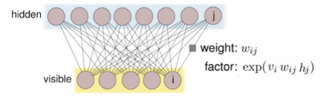
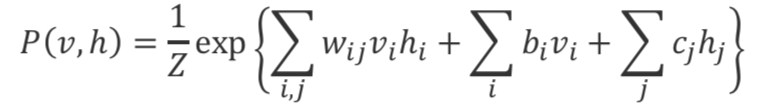
联合分布为：



单个数据点的对数似然度（不可观察的边际被边缘化）：



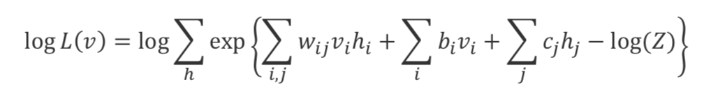
对数似然比的梯度 模型参数：



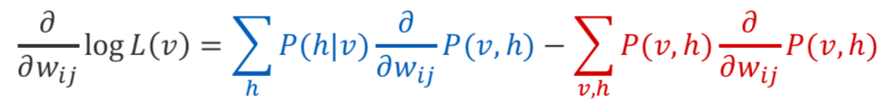
对数似然比的梯度 参数（替代形式）：



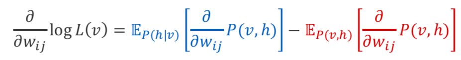
两种期望都可以通过抽样来近似， 从后部采样是准确的（RBM在给定的h上分解）。 通过MCMC从关节进行采样（例如，吉布斯采样）

在神经网络文献中：

• 计算第一项称为钳位/唤醒/正相（网络是“清醒的”，因为它取决于可见变量）
• 计算第二项称为非固定/睡眠/自由/负相（该网络“处于睡眠状态”，因为它对关节的可见变量进行了采样；比喻，它梦见了可见的输入）

通过随机梯度下降（SGD）优化给定数据的模型对数似然来完成学习， 第二项（负相）的估计严重依赖于马尔可夫链的混合特性，这经常导致收敛缓慢并且需要额外的计算。

II: Sigmoid Belief Networks



Sigimoid信念网是简单的贝叶斯网络，其二进制变量的条件概率由Sigmoid函数表示：



贝叶斯网络表现出一种称为“解释效应”的现象：如果A与C相关，则B与C相关的机会减少。 ⇒在给定C的情况下A和B相互关联。



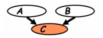
值得注意的是， 由于“解释效应”，当我们以信念网络中的可见层为条件时，所有隐藏变量都将成为因变量。

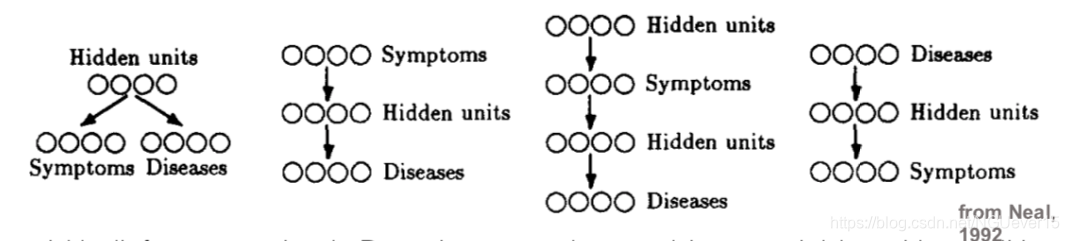
Sigmoid Belief Networks as graphical models

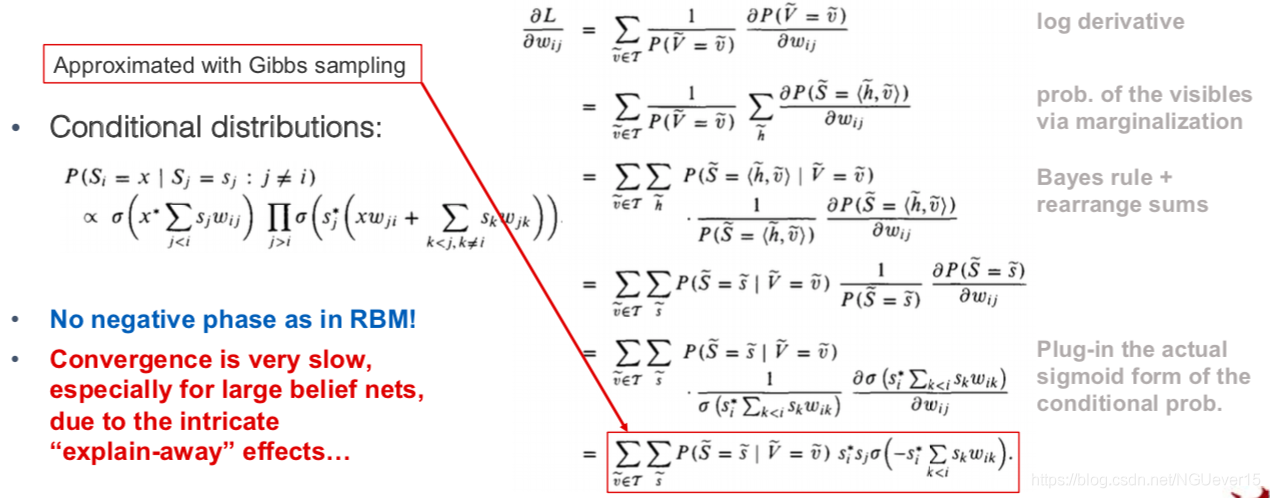
尼尔提出了用于学习和推理的蒙特卡洛方法（尼尔，1992年）：



RBMs are infinite belief networks

要对模型参数进行梯度更新，我们需要通过采样计算期望值。

• 我们可以在第一阶段从后验中精确采样
• 我们运行吉布斯块抽样，以从联合分布中近似抽取样本
  
  

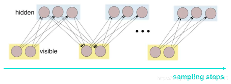
条件分布\(p(v| h)\)和\(p(h|v)\)用sigmoid表示， 因此，我们可以将以RBM表示的联合分布中的Gibbs采样视为无限深的Sigmoid信念网络中的自顶向下传播！



RBM等效于无限深的信念网络。当我们训练RBM时，实际上就是在训练一个无限深的简短网， 只是所有图层的权重都捆绑在一起。如果权重在某种程度上“统一”，我们将获得一个深度信仰网络。

Deep Belief Networks and Boltzmann Machines

III: Deep Belief Nets



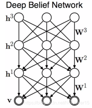
DBN是混合图形模型（链图）。其联合概率分布可表示为：

其中蕴含的挑战：

由于explaining away effect，因此在DBN中进行精确推断是有问题的

训练分两个阶段进行：

• 贪婪的预训练+临时微调； 没有适当的联合训练
• 近似推断为前馈（自下而上）

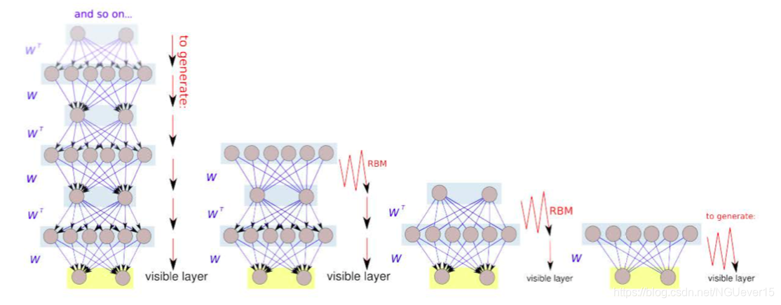
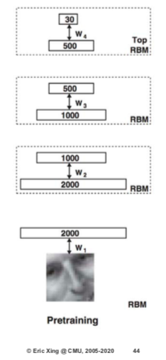
Layer-wise pre-training

• 预训练并冻结第一个RBM
• 在顶部堆叠另一个RBM并对其进行训练
• 重物2层以上的重物保持绑紧状态
• 我们重复此过程：预训练和解开

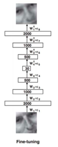
Fine-tuning

• Pre-training is quite ad-hoc（特别指定） and is unlikely to lead to a good probabilistic model per se
• However, the layers of representations could perhaps be useful for some other downstream tasks!
• We can further “fine-tune” a pre-trained DBN for some other task

Setting A: Unsupervised learning (DBN → autoencoder)

1. Pre-train a stack of RBMs in a greedy layer-wise fashion
2. “Unroll” the RBMs to create an autoencoder
3. Fine-tune the parameters by optimizing the reconstruction error（重构误差）

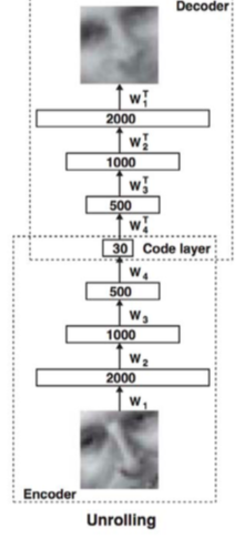
Setting B: Supervised learning (DBN → classifier)

1. Pre-train a stack of RBMs in a greedy layer-wise fashion
2. “Unroll” the RBMs to create a feedforward classifier
3. Fine-tune the parameters by optimizing the reconstruction error

Deep Belief Nets and Boltzmann Machines



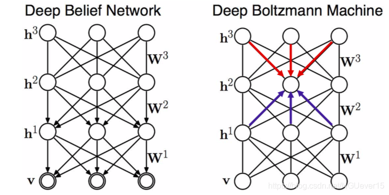
DBMs are fully un-directed models (Markov random fields). Can be trained similarly as RBMs via MCMC (Hinton & Sejnowski, 1983). Use a variational approximation(变分近似) of the data distribution for faster training (Salakhutdinov & Hinton, 2009). Similarly, can be used to initialize other networks for downstream tasks

A few critical points to note about all these models:

• The primary goal of deep generative models is to represent the distribution of the observable variables. Adding layers of hidden variables allows to represent increasingly more complex distributions.
• Hidden variables are secondary (auxiliary) elements used to facilitate learning of complex dependencies between the observables.
• Training of the model is ad-hoc, but what matters is the quality of learned hidden representations.
• Representations are judged by their usefulness on a downstream task (the probabilistic meaning of the model is often discarded at the end).
• In contrast, classical graphical models are often concerned with the correctness of learning and inference of all variables

Conclusion

• DL & GM: the fields are similar in the beginning (structure, energy, etc.), and then diverge to their own signature pipelines
• DL: most effort is directed to comparing different architectures and their components (models are driven by evaluating empirical performance on a downstream tasks)
• DL models are good at learning robust hierarchical representations from the data and suitable for simple reasoning (call it “low-level cognition”)
• GM: the effort is directed towards improving inference accuracy and convergence speed
• GMs are best for provably correct inference and suitable for high-level complex reasoning tasks (call it “high-level cognition”) 推理任务
• Convergence of both fields is very promising!

03 Combining DL methods and GMs

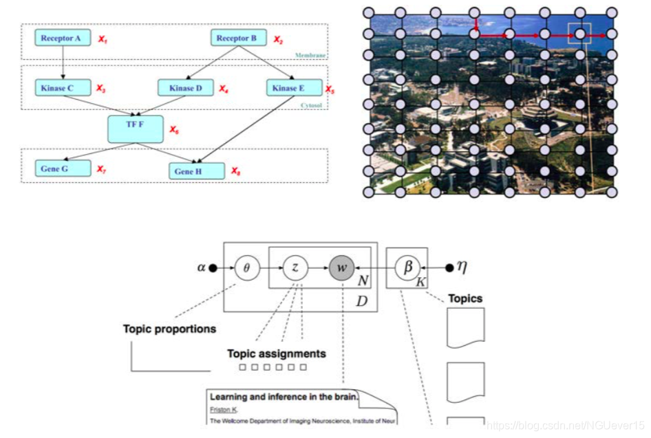
Using outputs of NNs as inputs to GMs

Combining sequential NNs and GMs

HMM：隐马尔可夫



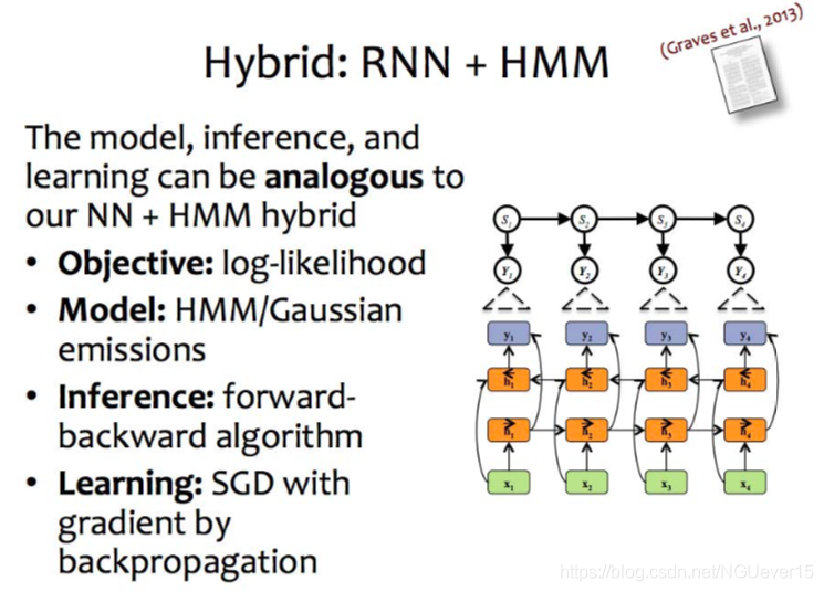
Hybrid NNs + conditional GMs



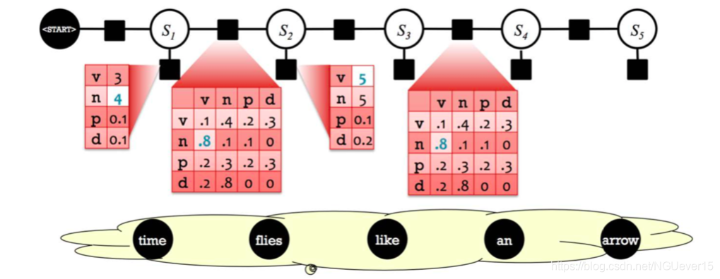
In a standard CRF条件随机场, each of the factor cells is a parameter.

In a hybrid model, these values are computed by a neural network.

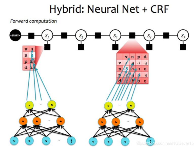
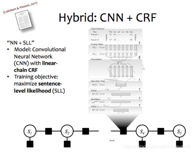
GMs with potential functions represented by NNs q NNs with structured outputs

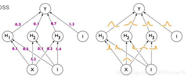
Using GMs as Prediction Explanations

!!!! How do we build a powerful predictive model whose predictions we can interpret in terms of semantically meaningful features?

Contextual Explanation Networks (CENs)

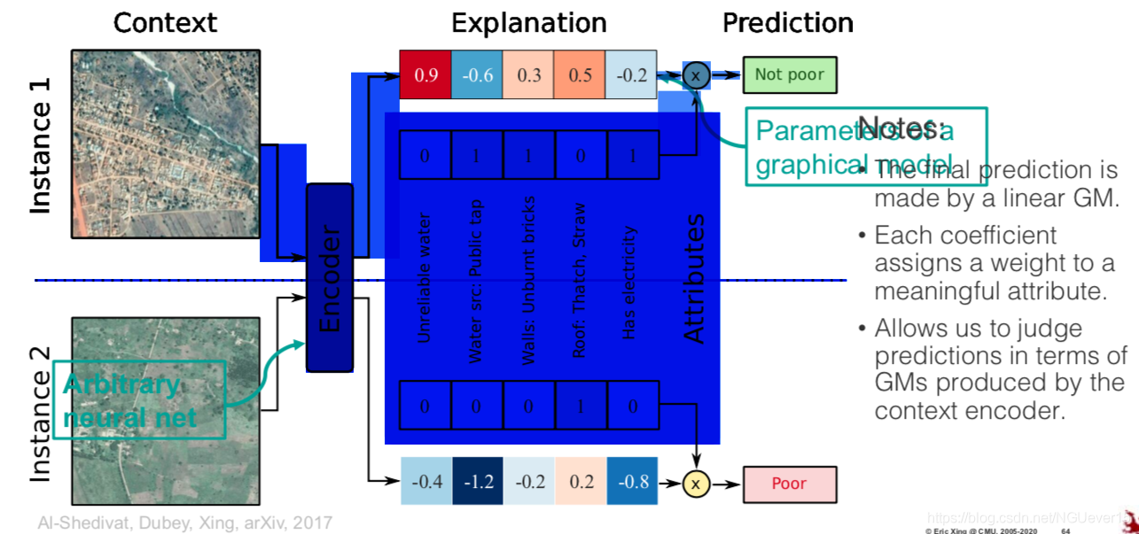
• The final prediction is made by a linear GM.
• Each coefficient assigns a weight to a meaningful attribute.
• Allows us to judge predictions in terms of GMs produced by the context encoder.

CEN: Implementation Details



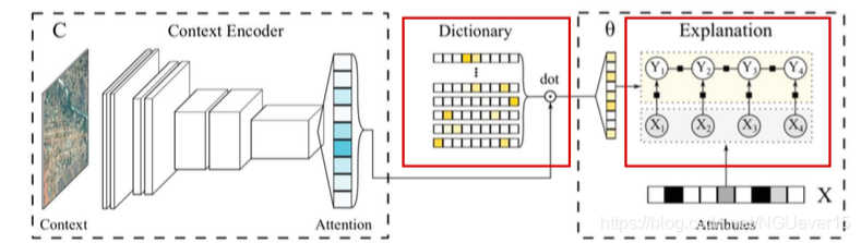
Workflow:

• Maintain a (sparse稀疏) dictionary of GM parameters.
• Process complex inputs (images, text, time series, etc.) using deep nets; use soft attention to either select or combine models from the dictionary.
  
  • Use constructed GMs (e.g., CRFs) to make predictions.
  
  • Inspect GM parameters to understand the reasoning behind predictions.

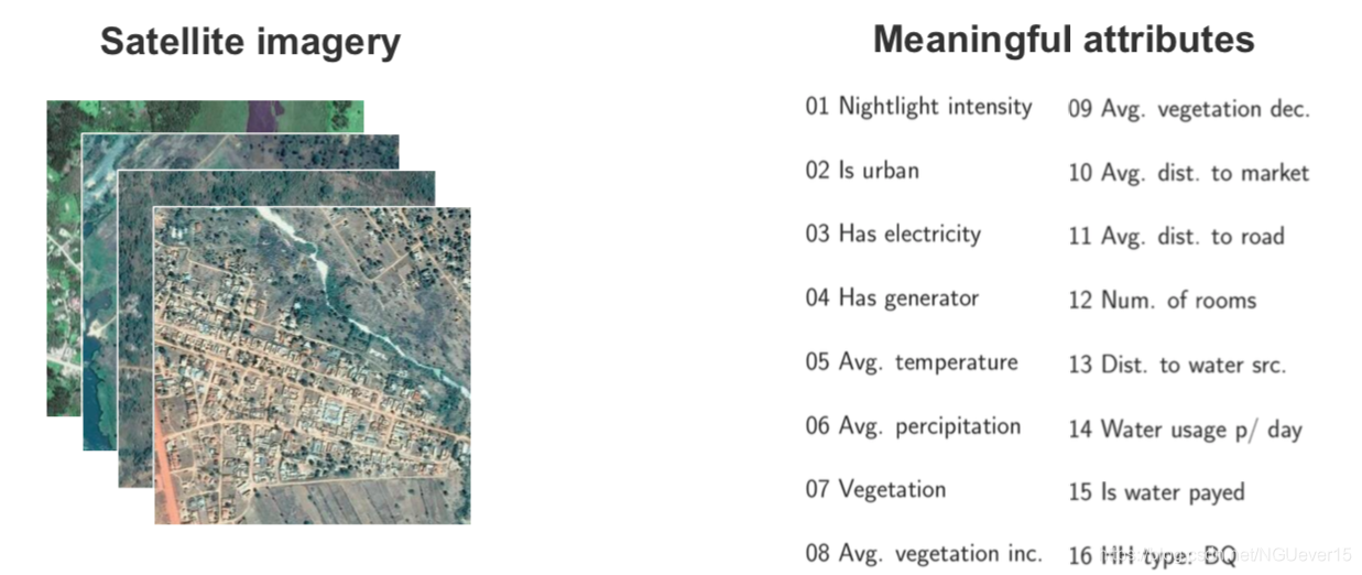
Results: imagery as context



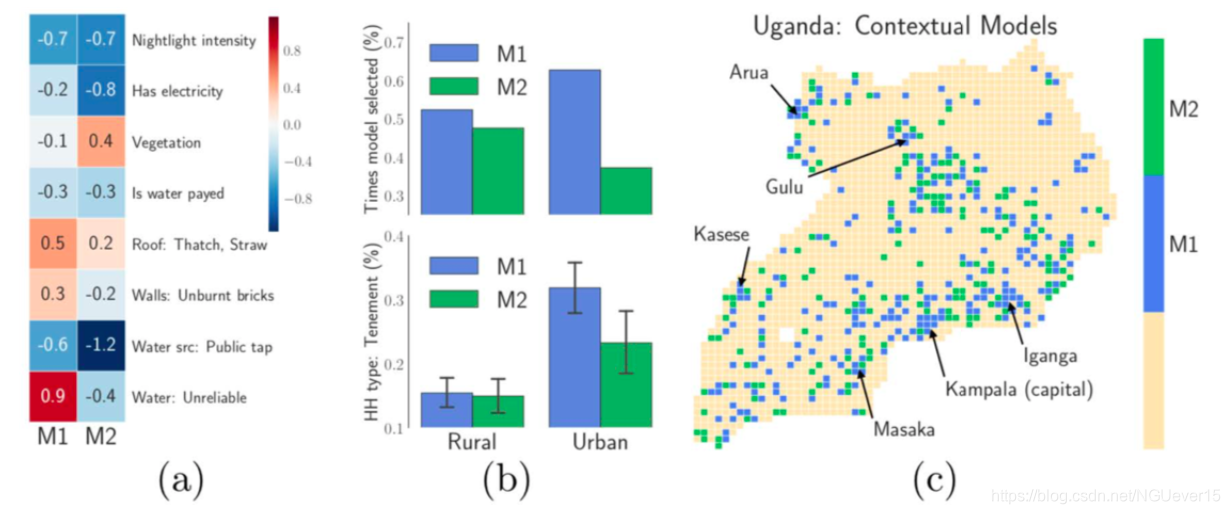
Based on the imagery, CEN learns to select different models for urban and rural

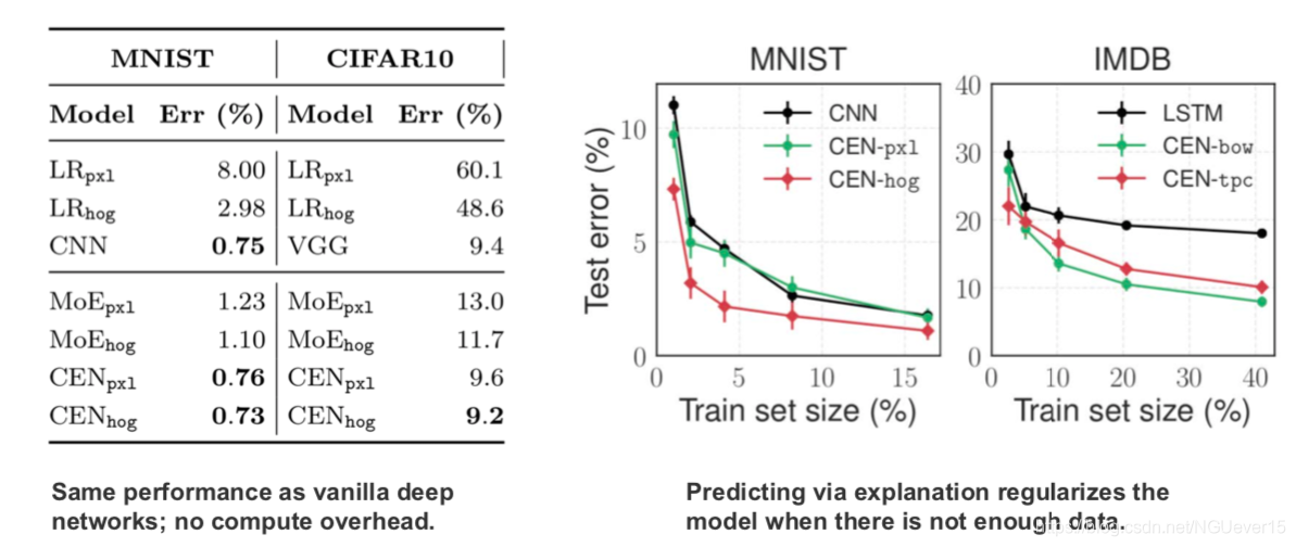
Results: classical image & text datasets



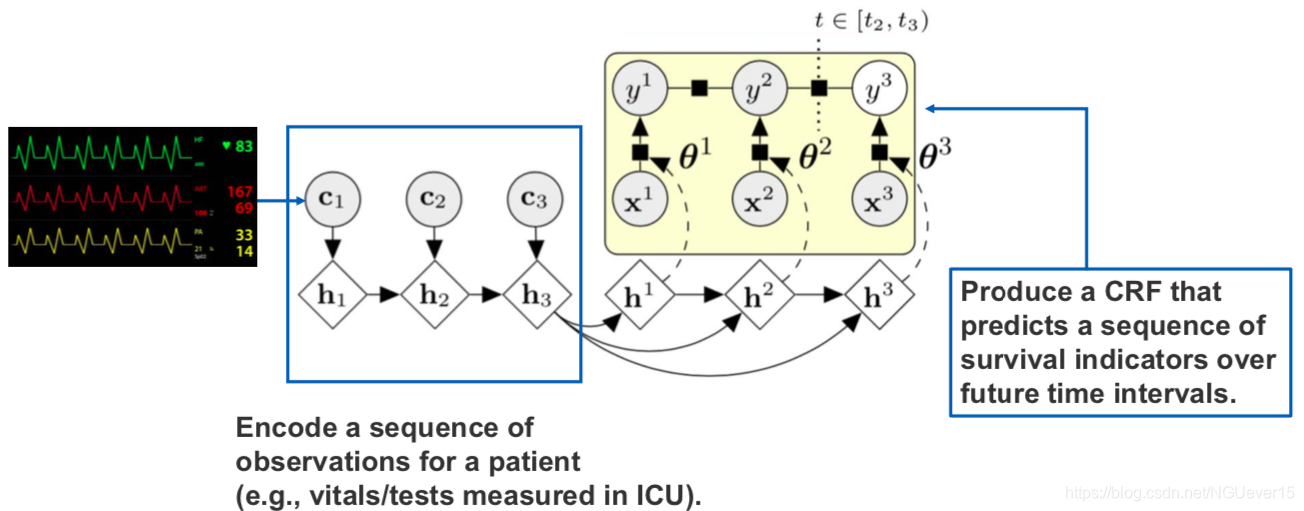
CEN architectures for survival analysis

04 Bayesian Learning of NNs

Bayesian learning of NN parameters q Deep kernel learning

A neural network as a probabilistic model: Likelihood: \(p(y|x, \theta)\)

• Categorical distribution for classification ⇒ cross-entropy loss 交叉熵损失
• Gaussian distribution for regression ⇒ squared loss平方损失
• Gaussianprior⇒L2regularization
• Laplaceprior⇒L1regularization

Bayesian learning [MacKay 1992, Neal 1996, de Freitas 2003]