花授粉优化算法-python/matlab

import numpy as np
from matplotlib import pyplot as plt
import random                                                                                        

# 初始化种群
def init(n_pop, lb, ub, nd):
    """
    :param n_pop: 种群
    :param lb: 下界
    :param ub: 上界
    :param nd: 维数
    """
    p = lb + (ub - lb) * np.random.rand(n_pop, nd)
    return p                                                                                           

# 适应度函数
def sphere(x):
    y = np.sum(x ** 2, 1)
    return y                                                                                           

def Ackley_1(x):
    n, d = x.shape
    y = -20 * np.exp(-0.02 * np.sqrt(1 / d * np.sum(x ** 2, 1))) - np.exp(
        1 / d * np.sum(np.cos(2 * np.pi * x), 1)) + 20 + np.e
    return y                                                                                           

def Ackley_2(x):
    y = -200 * np.exp(-0.02 * np.sqrt(x[:, 0] ** 2 + x[:, 1] ** 2))
    return y                                                                                           

def Ackley_3(x):
    y = -200 * np.exp(-0.02 * np.sqrt(x[:, 0] ** 2 + x[:, 1] ** 2)) + 5 * np.exp(
        np.cos(3 * x[:, 0]) + np.sin(3 * x[:, 1]))
    return y                                                                                           

def Ackley_4(x, y=0):
    _, d = x.shape
    for i in range(1, d):
        y += np.exp(-0.2 * np.sqrt(x[:, i - 1] ** 2 + x[:, i] ** 2)) + 3 * (
                np.cos(2 * x[:, i - 1]) + np.sin(2 * x[:, i]))
    return y                                                                                           

def Adjiman(x):
    y = np.cos(x[:, 0]) * np.sin(x[:, 1]) - x[:, 0] / (x[:, 1] ** 2 + 1)
    return y                                                                                           

def Alpine(x):
    y = np.sum(np.abs(x * np.sin(x) + 0.1 * x), 1)
    return y                                                                                           

def Alpine2(x):
    y = np.prod(np.sqrt(x) * np.sin(x), axis=1)
    return y                                                                                           

def Bartels(x):
    y = np.abs(x[:, 0] ** 2 + x[:, 1] ** 2 + x[:, 0] * x[:, 1]) + np.abs(np.sin(x[:, 0])) + np.abs(np.c
    return y                                                                                           

def Beale(x):
    y = (1.5 - x[:, 0] + x[:, 0] * x[:, 1]) ** 2 + (2.25 - x[:, 0] + x[:, 0] * x[:, 1] ** 2) ** 2 + (
            2.625 - x[:, 0] + x[:, 0] * x[:, 1] ** 3) ** 2
    return y                                                                                           

f_score = sphere  # 函数句柄                                                                               

# Levy飞行Beale
def Levy(nd, beta=1.5):
    num = np.random.gamma(1 + beta) * np.sin(np.pi * beta / 2)
    den = np.random.gamma((1 + beta) / 2) * beta * 2 ** ((beta - 1) / 2)
    sigma_u = (num / den) ** (1 / beta)                                                                

    u = np.random.normal(0, sigma_u ** 2, (1, nd))
    v = np.random.normal(0, 1, (1, nd))                                                                

    z = u / (np.abs(v) ** (1 / beta))
    return z                                                                                           

def FPA(Max_g, n_pop, Pop, nd, lb, ub, detail):  # FPA算法
    """
    :param Max_g: 迭代次数
    :param n_pop: 种群数目
    :param Pop: 花粉配子
    :param nd: 维数
    :param lb: 下界
    :param ub: 上界
    :param detail: 显示详细信息
    """
    # 计算初始种群中最好个体适应度值
    pop_score = f_score(Pop)
    g_best = np.min(pop_score)
    g_best_loc = np.argmin(pop_score)
    g_best_p = Pop[g_best_loc, :].copy()                                                               

    # 问题设置
    p = 0.8
    best_fit = np.empty((Max_g,))
    # 迭代
    for it in range(1, Max_g + 1):
        for i in range(n_pop):
            if np.random.rand() < p:
                new_pop = Pop[i, :] + Levy(nd) * (g_best_p - Pop[i, :])
                new_pop = np.clip(new_pop, lb, ub)  # 越界处理
            else:
                idx = random.sample(list(range(n_pop)), 2)
                new_pop = Pop[i, :] + np.random.rand() * (Pop[idx[1], :] - Pop[idx[0], :])
                new_pop = np.clip(new_pop, lb, ub)  # 越界处理
            if f_score(new_pop.reshape((1, -1))) < f_score(Pop[i, :].reshape((1, -1))):
                Pop[i, :] = new_pop
        # 计算更新后种群中最好个体适应度值
        pop_score = f_score(Pop)
        new_g_best = np.min(pop_score)
        new_g_best_loc = np.argmin(pop_score)                                                          

        if new_g_best < g_best:
            g_best = new_g_best
            g_best_p = Pop[new_g_best_loc, :].copy()
        best_fit[it - 1] = g_best                                                                      

        if detail:
            print("----------------{}/{}--------------".format(it, Max_g))
            print(g_best)
            print(g_best_p)                                                                            

    return best_fit, g_best                                                                            

if __name__ == "__main__":
    pop = init(30, -100, 100, 2)
    fitness, g_best = FPA(1000, 30, pop, 2, -100, 100, True)                                           

    # 可视化
    plt.figure()
    # plt.plot(fitness)
    plt.semilogy(fitness)
    # 可视化
    # fig = plt.figure()
    # plt.plot(p1, fit)
    plt.show()                                                                                         

花授粉算法Matlab代码
% 清屏和工作空间变量
clc
clear
Step 1:    问题定义
npop = 30;    % 种群数目
dpop = 2;     % 种群维数
ub = 100;     % 种群的上界
lb = -100;    % 种群的下界
Step 2： 初始化种群
pop = lb + rand(npop, dpop).*(ub - lb);  % pop是初始种群
Step 3：适应度函数
fScore = @ sphere
Step 4：Levy飞行
levy = @ Levy
Step 5：计算初始种群最好的适应度值
popScore = fScore(pop);
[bestscore, loc] = min(popScore);
bestpop = pop(loc, :);
Step 6：参数设置
iterMax = 1000;  %  最大迭代次数
p = 0.8;  %  转换概率
BestScore = ones(iterMax, 1);
Step 7：越界处理
Clip = @ clip;  % 越界处理函数
Step 8：迭代
for it=1:iterMax
    for i = 1:npop
        if rand < p
            newpop = pop(i, :) + levy(1, dpop).*(bestpop - pop(i, :));  % 异花授粉
        else
            idx = randsample(30, 2);
            newpop = pop(i, :) + rand*(pop(idx(1), :) - pop(idx(2), :));  % 自花授粉
        end
        newpop = Clip(newpop, ub, lb);  % 越界处理
        if fScore(newpop) < fScore(pop(i, :))
            pop(i, :) = newpop;  % 更新种群
        end
    end
    popScore = fScore(pop);
    [newBestScore, Loc] = min(popScore);
    if newBestScore < bestscore
        bestscore = newBestScore;
        bestpop = pop(loc, :);
    end
    BestScore(it) = bestscore;
    disp(['Iteration ' num2str(it) ': Best Cost = ' num2str(bestscore)]);
    disp(['Bestpop ' num2str(bestpop)])
end
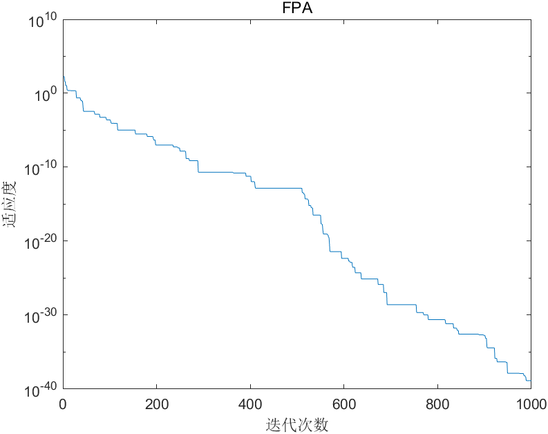
Step 9：可视化
figure
semilogy(BestScore)
% plot(BestScore)
xlim([0 1000])
xlabel('迭代次数')
ylabel('适应度')
title('FPA')

function L=Levy(d)
%% Levy飞行
    beta=3/2;
    sigma=(gamma(1+beta)*sin(pi*beta/2)/(gamma((1+beta)/2)*beta*2^((beta-1)/2)))^(1/beta);
    u=random('normal', 0, sigma, 1, d);
    v=random('normal', 0, 1, 1, d);
    L=0.01*u./abs(v).^(1/beta);
end

function s=simplebounds(s,Lb,Ub)
%% 越界处理函数
    ns_tmp=s;
    I=ns_tmp<Lb;
    ns_tmp(I)=Lb(I);
    J=ns_tmp>Ub;
    ns_tmp(J)=Ub(J);
    s=ns_tmp;
end

function [y] = Sphere(xx)
%% 目标函数
    d = length(xx);
    sum = 0;
    for ii = 1:d
        xi = xx(ii);
        sum = sum + xi^2;
    end

    y = sum;
end