【机器学习】用Octave实现一元线性回归的梯度下降算法

Step1 Plotting the Data

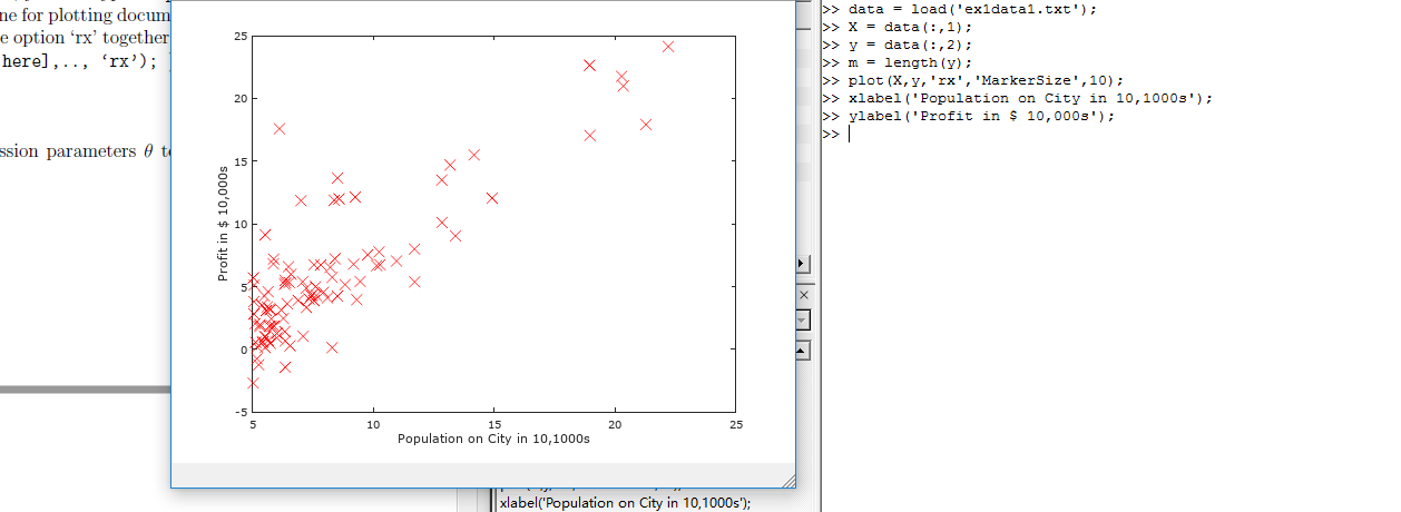
在处理数据之前，我们通常要了解数据，对于这次的数据集合，我们可以通过离散的点来描绘它，在一个2D的平面里把它画出来。

6.1101,17.592
5.5277,9.1302
8.5186,13.662
7.0032,11.854
5.8598,6.8233
8.3829,11.886
7.4764,4.3483
8.5781,12
6.4862,6.5987
5.0546,3.8166
5.7107,3.2522
14.164,15.505
5.734,3.1551
8.4084,7.2258
5.6407,0.71618
5.3794,3.5129
6.3654,5.3048
5.1301,0.56077
6.4296,3.6518
7.0708,5.3893
6.1891,3.1386
20.27,21.767
5.4901,4.263
6.3261,5.1875
5.5649,3.0825
18.945,22.638
12.828,13.501
10.957,7.0467
13.176,14.692
22.203,24.147
5.2524,-1.22
6.5894,5.9966
9.2482,12.134
5.8918,1.8495
8.2111,6.5426
7.9334,4.5623
8.0959,4.1164
5.6063,3.3928
12.836,10.117
6.3534,5.4974
5.4069,0.55657
6.8825,3.9115
11.708,5.3854
5.7737,2.4406
7.8247,6.7318
7.0931,1.0463
5.0702,5.1337
5.8014,1.844
11.7,8.0043
5.5416,1.0179
7.5402,6.7504
5.3077,1.8396
7.4239,4.2885
7.6031,4.9981
6.3328,1.4233
6.3589,-1.4211
6.2742,2.4756
5.6397,4.6042
9.3102,3.9624
9.4536,5.4141
8.8254,5.1694
5.1793,-0.74279
21.279,17.929
14.908,12.054
18.959,17.054
7.2182,4.8852
8.2951,5.7442
10.236,7.7754
5.4994,1.0173
20.341,20.992
10.136,6.6799
7.3345,4.0259
6.0062,1.2784
7.2259,3.3411
5.0269,-2.6807
6.5479,0.29678
7.5386,3.8845
5.0365,5.7014
10.274,6.7526
5.1077,2.0576
5.7292,0.47953
5.1884,0.20421
6.3557,0.67861
9.7687,7.5435
6.5159,5.3436
8.5172,4.2415
9.1802,6.7981
6.002,0.92695
5.5204,0.152
5.0594,2.8214
5.7077,1.8451
7.6366,4.2959
5.8707,7.2029
5.3054,1.9869
8.2934,0.14454
13.394,9.0551
5.4369,0.61705

ex1data1.txt

我们把ex1data1中的内容读取到X变量和y变量中，用m表示数据长度。

data = load('ex1data1.txt');
X = data(:,1);
y = data(:,2);
m = length(y);

接下来通过图像描绘出来。

plot(x,y,'rx','MakerSize',10);
ylabel('Profit in $10,000s');
xlabel('Population of City in 10,000s');

　　现在我们得到图像如图所示，就是原始的数据的直观表示。

Step2 Gradient Descent

现在，我们通过梯度下降法对参数θ进行线性回归。

依照我们之前所得出步骤方法

迭代更新

计算θ值函数：

function J = computeCost(X, y, theta)
%COMPUTECOST Compute cost for linear regression
%   J = COMPUTECOST(X, y, theta) computes the cost of using theta as the
%   parameter for linear regression to fit the data points in X and y

% Initialize some useful values
m = length(y); % number of training examples

% You need to return the following variables correctly
J = 0;

% ====================== YOUR CODE HERE ======================
% Instructions: Compute the cost of a particular choice of theta
%               You should set J to the cost.
J = sum((X * theta - y).^2) / (2*m);     % X(79,2)  theta(2,1)

% =========================================================================

end

　　接下来是梯度下降函数

function [theta, J_history] = gradientDescent(X, y, theta, alpha, num_iters)
%GRADIENTDESCENT Performs gradient descent to learn theta
%   theta = GRADIENTDESENT(X, y, theta, alpha, num_iters) updates theta by
%   taking num_iters gradient steps with learning rate alpha

% Initialize some useful values
m = length(y); % number of training examples
J_history = zeros(num_iters, 1);
theta_s=theta;

for iter = 1:num_iters

    % ====================== YOUR CODE HERE ======================
    % Instructions: Perform a single gradient step on the parameter vector
    %               theta.
    %
    % Hint: While debugging, it can be useful to print out the values
    %       of the cost function (computeCost) and gradient here.
    %
    theta(1) = theta(1) - alpha / m * sum(X * theta_s - y);
    theta(2) = theta(2) - alpha / m * sum((X * theta_s - y) .* X(:,2));
% 必须同时更新theta(1)和theta(2)，所以不能用X * theta,而要用theta_s存储上次结果。
    theta_s=theta; 

    % ============================================================

    % Save the cost J in every iteration
    J_history(iter) = computeCost(X, y, theta);

end
J_history
end

绘图函数：

function plotData(x, y)
%PLOTDATA Plots the data points x and y into a new figure
% PLOTDATA(x,y) plots the data points and gives the figure axes labels of
% population and profit.

% ====================== YOUR CODE HERE ======================
% Instructions: Plot the training data into a figure using the
% "figure" and "plot" commands. Set the axes labels using
% the "xlabel" and "ylabel" commands. Assume the
% population and revenue data have been passed in
% as the x and y arguments of this function.
%
% Hint: You can use the 'rx' option with plot to have the markers
% appear as red crosses. Furthermore, you can make the
% markers larger by using plot(..., 'rx', 'MarkerSize', 10);

figure; % open a new figure window
plot(x, y, 'rx', 'MarkerSize', 10); % Plot the data
ylabel('Profit in $10,000s'); % Set the y axis label
xlabel('Population of City in 10,000s'); % Set the x axis label

% ============================================================

end

　　　　根据以上函数，我们进行线性回归：

%% Machine Learning Online Class - Exercise 1: Linear Regression

%  Instructions
%  ------------
%
%  This file contains code that helps you get started on the
%  linear exercise. You will need to complete the following functions
%  in this exericse:
%
%     warmUpExercise.m
%     plotData.m
%     gradientDescent.m
%     computeCost.m
%     gradientDescentMulti.m
%     computeCostMulti.m
%     featureNormalize.m
%     normalEqn.m
%
%  For this exercise, you will not need to change any code in this file,
%  or any other files other than those mentioned above.
%
% x refers to the population size in 10,000s
% y refers to the profit in $10,000s
%

%% ==================== Part 1: Basic Function ====================
% Complete warmUpExercise.m
fprintf('Running warmUpExercise ... \n');
fprintf('5x5 Identity Matrix: \n');
warmUpExercise()

fprintf('Program paused. Press enter to continue.\n');
pause;

%% ======================= Part 2: Plotting =======================
fprintf('Plotting Data ...\n')
data = load('ex1data1.txt');
X = data(:, 1); y = data(:, 2);
m = length(y); % number of training examples

% Plot Data
% Note: You have to complete the code in plotData.m
plotData(X, y);

fprintf('Program paused. Press enter to continue.\n');
pause;

%% =================== Part 3: Gradient descent ===================
fprintf('Running Gradient Descent ...\n')

X = [ones(m, 1), data(:,1)]; % Add a column of ones to x
theta = zeros(2, 1); % initialize fitting parameters

% Some gradient descent settings
iterations = 1500;
alpha = 0.01;

% compute and display initial cost
computeCost(X, y, theta)

% run gradient descent
theta = gradientDescent(X, y, theta, alpha, iterations);

% print theta to screen
fprintf('Theta found by gradient descent: ');
fprintf('%f %f \n', theta(1), theta(2));

% Plot the linear fit
hold on; % keep previous plot visible
plot(X(:,2), X*theta, '-')
legend('Training data', 'Linear regression')
hold off % don't overlay any more plots on this figure

% Predict values for population sizes of 35,000 and 70,000
predict1 = [1, 3.5] *theta;
fprintf('For population = 35,000, we predict a profit of %f\n',...
    predict1*10000);
predict2 = [1, 7] * theta;
fprintf('For population = 70,000, we predict a profit of %f\n',...
    predict2*10000);

fprintf('Program paused. Press enter to continue.\n');
pause;

%% ============= Part 4: Visualizing J(theta_0, theta_1) =============
fprintf('Visualizing J(theta_0, theta_1) ...\n')

% Grid over which we will calculate J
theta0_vals = linspace(-10, 10, 100);
theta1_vals = linspace(-1, 4, 100);

% initialize J_vals to a matrix of 0's
J_vals = zeros(length(theta0_vals), length(theta1_vals));

% Fill out J_vals
for i = 1:length(theta0_vals)
    for j = 1:length(theta1_vals)
	  t = [theta0_vals(i); theta1_vals(j)];
	  J_vals(i,j) = computeCost(X, y, t);
    end
end

% Because of the way meshgrids work in the surf command, we need to
% transpose J_vals before calling surf, or else the axes will be flipped
J_vals = J_vals';
% Surface plot
figure;
surf(theta0_vals, theta1_vals, J_vals)
xlabel('\theta_0'); ylabel('\theta_1');

% Contour plot
figure;
% Plot J_vals as 15 contours spaced logarithmically between 0.01 and 100
contour(theta0_vals, theta1_vals, J_vals, logspace(-2, 3, 20))
xlabel('\theta_0'); ylabel('\theta_1');
hold on;
plot(theta(1), theta(2), 'rx', 'MarkerSize', 10, 'LineWidth', 2);

　　

如图所示，绘制出线性回归函数。

这时所绘制2D等高线图梯度下降表面图：

function [X_norm, mu, sigma] = featureNormalize(X)
%FEATURENORMALIZE Normalizes the features in X
%   FEATURENORMALIZE(X) returns a normalized version of X where
%   the mean value of each feature is 0 and the standard deviation
%   is 1. This is often a good preprocessing step to do when
%   working with learning algorithms.

% You need to set these values correctly
X_norm = X;
mu = zeros(1, size(X, 2));      % mean value 均值   size(X,2)  列数
sigma = zeros(1, size(X, 2));   % standard deviation  标准差

% ====================== YOUR CODE HERE ======================
% Instructions: First, for each feature dimension, compute the mean
%               of the feature and subtract it from the dataset,
%               storing the mean value in mu. Next, compute the
%               standard deviation of each feature and divide
%               each feature by it's standard deviation, storing
%               the standard deviation in sigma.
%
%               Note that X is a matrix where each column is a
%               feature and each row is an example. You need
%               to perform the normalization separately for
%               each feature.
%
% Hint: You might find the 'mean' and 'std' functions useful.
%
  mu = mean(X);       %  mean value
  sigma = std(X);     %  standard deviation
  X_norm  = (X - repmat(mu,size(X,1),1)) ./  repmat(sigma,size(X,1),1);

% ============================================================

end
function [theta, J_history] = gradientDescentMulti(X, y, theta, alpha, num_iters)
%GRADIENTDESCENTMULTI Performs gradient descent to learn theta
%   theta = GRADIENTDESCENTMULTI(x, y, theta, alpha, num_iters) updates theta by
%   taking num_iters gradient steps with learning rate alpha

% Initialize some useful values
m = length(y); % number of training examples
J_history = zeros(num_iters, 1);

for iter = 1:num_iters

    % ====================== YOUR CODE HERE ======================
    % Instructions: Perform a single gradient step on the parameter vector
    %               theta.
    %
    % Hint: While debugging, it can be useful to print out the values
    %       of the cost function (computeCostMulti) and gradient here.
    %
    theta = theta - alpha / m * X' * (X * theta - y); 

    % ============================================================

    % Save the cost J in every iteration
    J_history(iter) = computeCostMulti(X, y, theta);

end

end
function J = computeCostMulti(X, y, theta)
%COMPUTECOSTMULTI Compute cost for linear regression with multiple variables
%   J = COMPUTECOSTMULTI(X, y, theta) computes the cost of using theta as the
%   parameter for linear regression to fit the data points in X and y

% Initialize some useful values
m = length(y); % number of training examples

% You need to return the following variables correctly
J = 0;

% ====================== YOUR CODE HERE ======================
% Instructions: Compute the cost of a particular choice of theta
%               You should set J to the cost.
J = sum((X * theta - y).^2) / (2*m);    

% =========================================================================

end
function [theta] = normalEqn(X, y)
%NORMALEQN Computes the closed-form solution to linear regression
%   NORMALEQN(X,y) computes the closed-form solution to linear
%   regression using the normal equations.

theta = zeros(size(X, 2), 1);

% ====================== YOUR CODE HERE ======================
% Instructions: Complete the code to compute the closed form solution
%               to linear regression and put the result in theta.
%

% ---------------------- Sample Solution ----------------------

theta = pinv( X' * X ) * X' * y;

% -------------------------------------------------------------

% ============================================================

end
%% Machine Learning Online Class
%  Exercise 1: Linear regression with multiple variables
%
%  Instructions
%  ------------
%
%  This file contains code that helps you get started on the
%  linear regression exercise.
%
%  You will need to complete the following functions in this
%  exericse:
%
%     warmUpExercise.m
%     plotData.m
%     gradientDescent.m
%     computeCost.m
%     gradientDescentMulti.m
%     computeCostMulti.m
%     featureNormalize.m
%     normalEqn.m
%
%  For this part of the exercise, you will need to change some
%  parts of the code below for various experiments (e.g., changing
%  learning rates).
%

%% Initialization

%% ================ Part 1: Feature Normalization ================

%% Clear and Close Figures
clear ; close all; clc

fprintf('Loading data ...\n');

%% Load Data
data = load('ex1data2.txt');
X = data(:, 1:2);
y = data(:, 3);
m = length(y);

% Print out some data points
fprintf('First 10 examples from the dataset: \n');
fprintf(' x = [%.0f %.0f], y = %.0f \n', [X(1:10,:) y(1:10,:)]');

fprintf('Program paused. Press enter to continue.\n');
pause;

% Scale features and set them to zero mean
fprintf('Normalizing Features ...\n');

[X mu sigma] = featureNormalize(X);      % 均值0，标准差1

% Add intercept term to X
X = [ones(m, 1) X];

%% ================ Part 2: Gradient Descent ================

% ====================== YOUR CODE HERE ======================
% Instructions: We have provided you with the following starter
%               code that runs gradient descent with a particular
%               learning rate (alpha).
%
%               Your task is to first make sure that your functions -
%               computeCost and gradientDescent already work with
%               this starter code and support multiple variables.
%
%               After that, try running gradient descent with
%               different values of alpha and see which one gives
%               you the best result.
%
%               Finally, you should complete the code at the end
%               to predict the price of a 1650 sq-ft, 3 br house.
%
% Hint: By using the 'hold on' command, you can plot multiple
%       graphs on the same figure.
%
% Hint: At prediction, make sure you do the same feature normalization.
%

fprintf('Running gradient descent ...\n');

% Choose some alpha value
alpha = 0.01;
num_iters = 8500;

% Init Theta and Run Gradient Descent
theta = zeros(3, 1);
[theta, J_history] = gradientDescentMulti(X, y, theta, alpha, num_iters);

% Plot the convergence graph
figure;
plot(1:numel(J_history), J_history, '-b', 'LineWidth', 2);
xlabel('Number of iterations');
ylabel('Cost J');

% Display gradient descent's result
fprintf('Theta computed from gradient descent: \n');
fprintf(' %f \n', theta);
fprintf('\n');

% Estimate the price of a 1650 sq-ft, 3 br house
% ====================== YOUR CODE HERE ======================
% Recall that the first column of X is all-ones. Thus, it does
% not need to be normalized.
price = [1 (([1650 3]-mu) ./ sigma)] * theta ;
% ============================================================

fprintf(['Predicted price of a 1650 sq-ft, 3 br house ' ...
         '(using gradient descent):\n $%f\n'], price);

fprintf('Program paused. Press enter to continue.\n');
pause;

%% ================ Part 3: Normal Equations ================

fprintf('Solving with normal equations...\n');

% ====================== YOUR CODE HERE ======================
% Instructions: The following code computes the closed form
%               solution for linear regression using the normal
%               equations. You should complete the code in
%               normalEqn.m
%
%               After doing so, you should complete this code
%               to predict the price of a 1650 sq-ft, 3 br house.
%

%% Load Data
data = csvread('ex1data2.txt');
X = data(:, 1:2);
y = data(:, 3);
m = length(y);

% Add intercept term to X
X = [ones(m, 1) X];

% Calculate the parameters from the normal equation
theta = normalEqn(X, y);

% Display normal equation's result
fprintf('Theta computed from the normal equations: \n');
fprintf(' %f \n', theta);
fprintf('\n');

% Estimate the price of a 1650 sq-ft, 3 br house
% ====================== YOUR CODE HERE ======================
price = [1 1650 3] * theta ;

% ============================================================

fprintf(['Predicted price of a 1650 sq-ft, 3 br house ' ...
         '(using normal equations):\n $%f\n'], price);

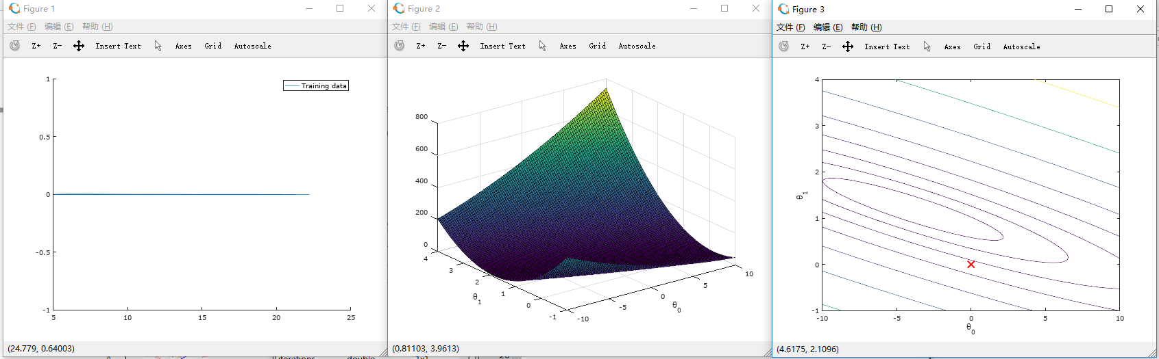
　　处理前：

处理后：

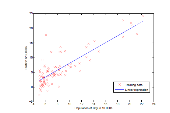
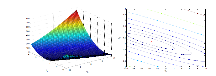
回归过程如图所示：

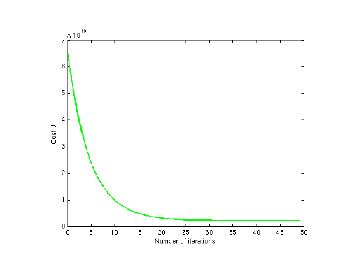
至此，我们通过梯度下降法解决了此问题，我们还可以通过之前所说的数学方法来解决，但是对于数据太大的情况（通常大于10000），我们就会通过梯度下降法来解决了

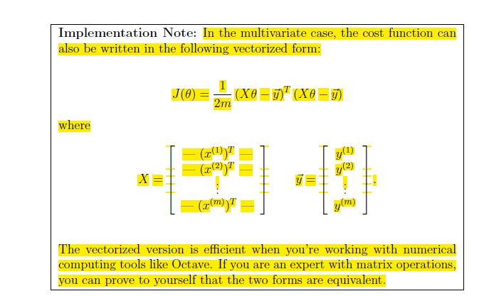
　　根据以上函数，我们进行线性回归：