《DSP using MATLAB》Problem 7.15

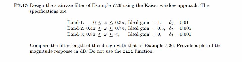
用Kaiser窗方法设计一个台阶状滤波器。

代码：

%% ++++++++++++++++++++++++++++++++++++++++++++++++++++++++++++++++++++++++++++++++
%%            Output Info about this m-file
fprintf('\n***********************************************************\n');
fprintf('        <DSP using MATLAB> Problem 7.15 \n\n');

banner();
%% ++++++++++++++++++++++++++++++++++++++++++++++++++++++++++++++++++++++++++++++++

% staircase bandpass 3-Band
w1 = 0;      w2 = 0.3*pi; delta1 = 0.01;
w3 = 0.4*pi; w4 = 0.7*pi; delta2 = 0.005;
w5 = 0.8*pi; w6 = pi;     delta3 = 0.001;

tr_width = min(w3-w2, w5-w3);

f = [0  w2  w3   w4   w5  w6]/pi;
m = [1  1   0.5  0.5  0   0];

[Rp1, As1] = delta2db(delta1, delta3);
[Rp2, As2] = delta2db(delta2, delta3);
As = min(As1, As2)

M = ceil((As-7.95)/(2.285*tr_width)) + 1;         % Kaiser Window Length

if As > 21 || As < 50
	beta = 0.5842*(As-21)^0.4 + 0.07886*(As-21);
else
	beta = 0.1102*(As-8.7);
end

fprintf('\nKaiser Window method, Filter Length: M = %d. beta = %.4f\n', M, beta);

n = [0:1:M-1]; wc1 = (w2+w3)/2; wc2 = (w4+w5)/2;

%wc = (ws + wp)/2,                    % ideal LPF cutoff frequency

hd = ideal_lp(wc1, M) + 0.5*(ideal_lp(wc2, M) - ideal_lp(wc1, M));
w_kai = (kaiser(M, beta))';  h = hd .* w_kai;
[db, mag, pha, grd, w] = freqz_m(h, [1]);  delta_w = 2*pi/1000;
[Hr,ww,P,L] = ampl_res(h);

Rp1 = -(min(db(1 :1: w2/delta_w+1)));                        % Actual Passband Ripple
fprintf('\nActual Passband Ripple1 is %.4f dB.\n', Rp1);

Rp2 = -(min(db(w3/delta_w+1 :1: w4/delta_w+1)));                        % Actual Passband Ripple
fprintf('\nActual Passband Ripple2 is %.4f dB.\n', Rp2);

As = -round(max(db(floor(w5/delta_w)+1 : 1 : floor(w6/delta_w)+1 )));   % Min Stopband attenuation
fprintf('\nMin Stopband attenuation is %.4f dB.\n', As);

[delta1, delta3] = db2delta(Rp1, As)
[delta2, delta3] = db2delta(Rp2, As)

% Plot

figure('NumberTitle', 'off', 'Name', 'Problem 7.15 ideal_lp Method')
set(gcf,'Color','white'); 

subplot(2,2,1); stem(n, hd); axis([0 M-1 -0.3 0.5]); grid on;
xlabel('n'); ylabel('hd(n)'); title('Ideal Impulse Response');

subplot(2,2,2); stem(n, w_kai); axis([0 M-1 0 1.1]); grid on;
xlabel('n'); ylabel('w(n)'); title('Kaiser Window');

subplot(2,2,3); stem(n, h); axis([0 M-1 -0.3 0.5]); grid on;
xlabel('n'); ylabel('h(n)'); title('Actual Impulse Response');

subplot(2,2,4); plot(w/pi, db); axis([0 1 -120 10]); grid on;
set(gca,'YTickMode','manual','YTick',[-90,-65,-6,0]);
set(gca,'YTickLabelMode','manual','YTickLabel',['90';'65';' 6';' 0']);
set(gca,'XTickMode','manual','XTick',[f]);
xlabel('frequency in \pi units'); ylabel('Decibels'); title('Magnitude Response in dB');

figure('NumberTitle', 'off', 'Name', 'Problem 7.15 h(n) ideal_lp Method')
set(gcf,'Color','white'); 

subplot(2,2,1); plot(w/pi, db); grid on; axis([0 2 -120 10]);
xlabel('frequency in \pi units'); ylabel('Decibels'); title('Magnitude Response in dB');
set(gca,'YTickMode','manual','YTick',[-90,-65,-6,0])
set(gca,'YTickLabelMode','manual','YTickLabel',['90';'65';' 6';' 0']);
set(gca,'XTickMode','manual','XTick',[f,1+f(2:6)]);

subplot(2,2,3); plot(w/pi, mag); grid on; %axis([0 2 -100 10]);
xlabel('frequency in \pi units'); ylabel('Absolute'); title('Magnitude Response in absolute');
set(gca,'XTickMode','manual','XTick',[f,1+f(2:6)]);
set(gca,'YTickMode','manual','YTick',[0,0.5, 1])

subplot(2,2,2); plot(w/pi, pha); grid on; %axis([0 1 -100 10]);
xlabel('frequency in \pi units'); ylabel('Rad'); title('Phase Response in Radians');
subplot(2,2,4); plot(w/pi, grd*pi/180);  grid on; %axis([0 1 -100 10]);
xlabel('frequency in \pi units'); ylabel('Rad'); title('Group Delay');

figure('NumberTitle', 'off', 'Name', 'Problem 7.15 Amp Res of h(n)')
set(gcf,'Color','white'); 

plot(ww/pi, Hr); grid on; %axis([0 1 -100 10]);
xlabel('frequency in \pi units'); ylabel('Hr'); title('Amplitude Response');
set(gca,'YTickMode','manual','YTick',[-delta3,0,delta3,0.5-0.005, 0.5+0.005,1-delta1,1,1+delta1])
%set(gca,'YTickLabelMode','manual','YTickLabel',['90';'45';' 0']);
set(gca,'XTickMode','manual','XTick',[f,2]);

%% +++++++++++++++++++++++++++++++++++++++++++++++++
%%                 fir2 function method
%% +++++++++++++++++++++++++++++++++++++++++++++++++
f = [w1, w2, w3, w4, w5, w6]/pi;
m = [1   1  0.5  0.5  0  0];
ripple = [0.01 0.005 0.001];

fprintf('\n--------- use fir2 function ---------\n');

h_check = fir2(M-1, f, m, kaiser(M, beta));

[db, mag, pha, grd, w] = freqz_m(h_check, [1]);
%[Hr,ww,P,L] = ampl_res(h_check);
[Hr,ww,P,L] = Hr_Type2(h_check);

%% -------------------------------------------
%%              plot
%% -------------------------------------------
figure('NumberTitle', 'off', 'Name', 'Problem 7.15 fir2 Method')
set(gcf,'Color','white'); 

subplot(2,2,1); stem(n, hd); axis([0 M-1 -0.3 0.5]); grid on;
xlabel('n'); ylabel('hd(n)'); title('Ideal Impulse Response');

subplot(2,2,2); stem(n, w_kai); axis([0 M-1 0 1.1]); grid on;
xlabel('n'); ylabel('w(n)'); title('Kaiser Window');

subplot(2,2,3); stem([0:M-1], h_check); axis([0 M -0.3 0.5]); grid on;
set(gca,'XTickMode','manual','XTick',[0 M/2 M]);
xlabel('n'); ylabel('h\_check(n)'); title('Actual Impulse Response');

subplot(2,2,4); plot(w/pi, db); axis([0 1 -120 10]); grid on;
set(gca,'YTickMode','manual','YTick',[-90,-65,-6,0]);
set(gca,'YTickLabelMode','manual','YTickLabel',['90';'65';' 6';' 0']);
set(gca,'XTickMode','manual','XTick',[f]);
xlabel('frequency in \pi units'); ylabel('Decibels'); title('Magnitude Response in dB');

figure('NumberTitle', 'off', 'Name', 'Problem 7.15 h_check(n) fir2 Method')
set(gcf,'Color','white'); 

subplot(2,2,1); plot(w/pi, db); grid on; axis([0 2 -120 10]);
xlabel('frequency in \pi units'); ylabel('Decibels'); title('Magnitude Response in dB');
set(gca,'YTickMode','manual','YTick',[-90,-65,-6,0])
set(gca,'YTickLabelMode','manual','YTickLabel',['90';'65';' 6';' 0']);
set(gca,'XTickMode','manual','XTick',[f,1+f(2:6)]);

subplot(2,2,3); plot(w/pi, mag); grid on; %axis([0 2 -100 10]);
xlabel('frequency in \pi units'); ylabel('Absolute'); title('Magnitude Response in absolute');
set(gca,'XTickMode','manual','XTick',[f,1+f(2:6)]);
set(gca,'YTickMode','manual','YTick',[0,0.5, 1])

subplot(2,2,2); plot(w/pi, pha); grid on; %axis([0 1 -100 10]);
xlabel('frequency in \pi units'); ylabel('Rad'); title('Phase Response in Radians');
subplot(2,2,4); plot(w/pi, grd*pi/180);  grid on; %axis([0 1 -100 10]);
xlabel('frequency in \pi units'); ylabel('Rad'); title('Group Delay');

　　运行结果：

Kaiser窗长M=74，两个通带衰减分别为0.0079dB和6.0345dB，阻带最小衰减65dB>60dB，满足设计要求。

用理想低通滤波方法设计的结果，实际脉冲响应、幅度谱（dB单位）

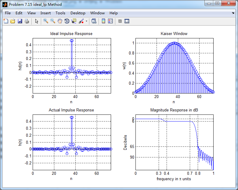
幅度谱（dB和绝对单位）、相位谱和群延迟响应

振幅响应（台阶状）

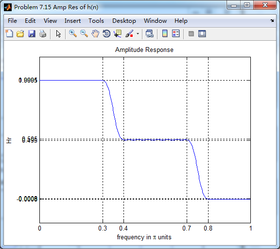
第一个台阶（通带）

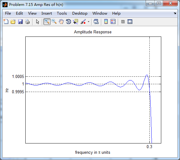
第二个台阶（通带）

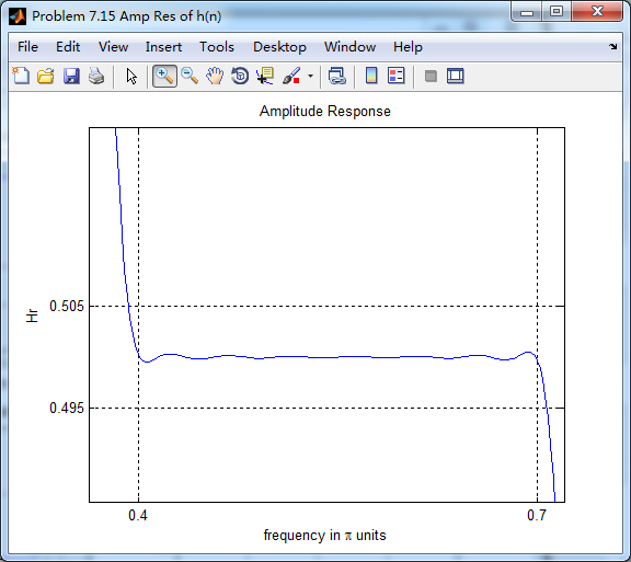
阻带

题目中暗示可以用fir1函数，但查了帮助和网上资料还是不会，只好用fir2函数的方法来设计，结果如下：

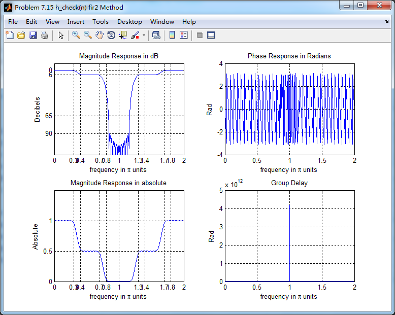
群延迟不是严格的常数了，非线性相位滤波器。