ML 逻辑回归 Logistic Regression

逻辑回归

Logistic Regression

1 分类 Classification

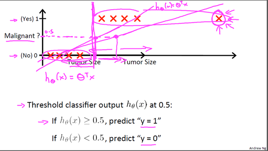
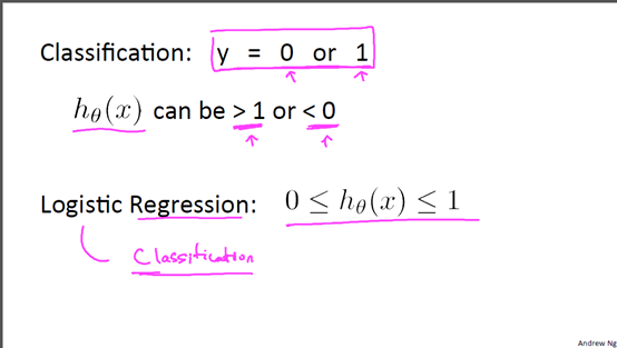
首先我们来看看使用线性回归来解决分类会出现的问题。下图中，我们加入了一个训练集，产生的新的假设函数使得我们进行分类出现了错误；而且线性回归计算的结果往往会远小于0或者远大于1，这对于0,1分类变得很奇怪。可见线性回归并不适用与分类。下面介绍的逻辑回归的结果总是在[0,1]，适用于分类，其实逻辑回归是一种分类算法。

2 假设函数Hypothesis Representation

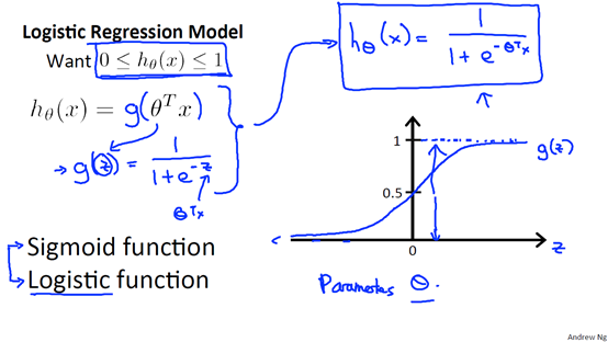
逻辑回归假设函数为：

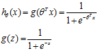
其中 是参数向量，特征向量。该函数叫做Logistic function（也叫做Sigmoid function）。函数图像如下，范围(0,1)

对于分类问题，它可以表示给定特征，参数属于类别1的概率，那么属于另一类的概率自然也就是。

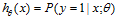
3 决策边界Decision Boundary

根据逻辑函数的特性可以看出，当，当

我们把 就称为决策边界（Decision Boundary）。

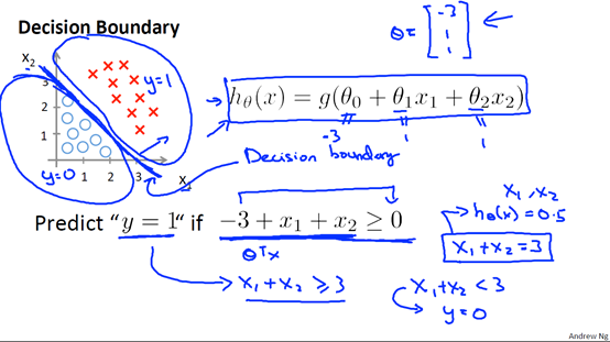
我们可以通过多项式组合来制定更加复杂的决策边界。

4 代价函数 Cost Function

代价函数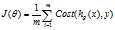 ，在线性回归中，我们的，如果在逻辑回归中也使用这个函数，那么代价函数会是一个非凸函数，无法使用梯度下降去求解参数，所以我们要寻找一些函数使得代价函数为凸函数。

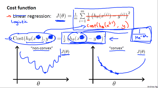
我们来看一下这个代价函数：

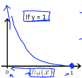
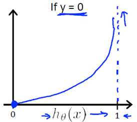
我们可以将它合并为一个公式：

5 梯度下降 Gradient Desecent

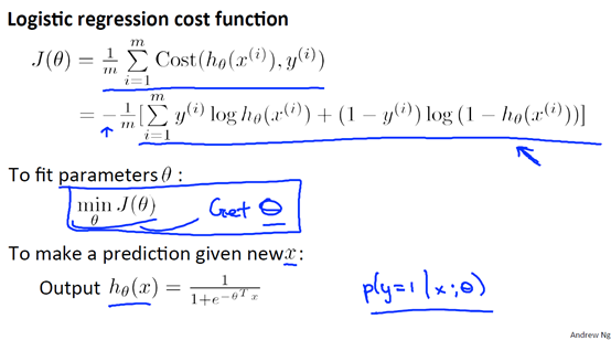
这里我们把代价函数写成这种形式是由最大似然估计得到了，当然也还有其他的形式。

梯度下降算法：

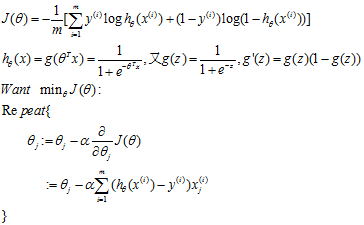
可以看到这里推导出来的公式看起来和线性回归梯度下降中推导出来的公式是一样的，但是要注意已经是sigmod函数而不是线性公式了，所以他们是两码事。

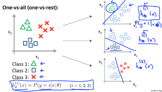
6 多分类 Multi-class classification: one-vs-all

我们可以降逻辑回归用于多分类问题，假设有K类，我们可以训练出K个分类器，每个分类器，将其中一种类别作为正类，其余的都是负类来训练，然后再预测时，类别属于概率最大的那个类。

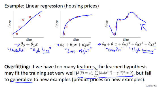
7 正则化regularization

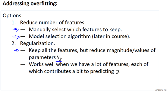
7.1 过拟合 overfitting

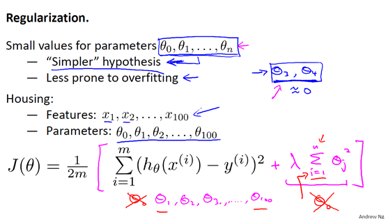
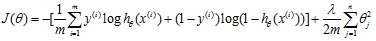
7.2 代价函数cost function

在代价函数中加入正则项，注意，这里对计算，而不是从开始。其中是正则项参数，如果太大，那么 会趋向于0，使得 ，导致欠拟合。

7.3 正则化线性回归 Regularized linear regression

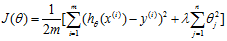
代价函数：

Gradeint descent

Repeat{

}

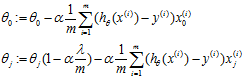
这里是一个比1小一点点的数。

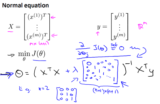
在线性回归中，我们除了梯度下降，还有正规方程的方法，正规方法加入正则项后：

7.4 正则化逻辑回归Regularized logistic regression

代价函数：

Gradient descent

Repeat{

}

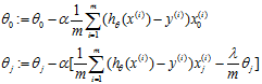
实验代码

正则化逻辑回归

 function [J, grad] = costFunctionReg(theta, X, y, lambda)
 %COSTFUNCTIONREG Compute cost and gradient for logistic regression with regularization
 %   J = COSTFUNCTIONREG(theta, X, y, lambda) computes the cost of using
 %   theta as the parameter for regularized logistic regression and the
 %   gradient of the cost w.r.t. to the parameters. 

 % Initialize some useful values
 m = length(y); % number of training examples

 % You need to return the following variables correctly
 J = ;
 grad = zeros(size(theta));

 % ====================== YOUR CODE HERE ======================
 % Instructions: Compute the cost of a particular choice of theta.
 %               You should set J to the cost.
 %               Compute the partial derivatives and set grad to the partial
 %               derivatives of the cost w.r.t. each parameter in theta
 hx=sigmoid(X*theta);
 Jnorm=(-/m)*(y'*log(hx)+(1-y)'*log(-hx));
 theta0=theta(); %注意theta0不用正则化
 theta1=theta(:end);
 Jreg=(lambda/(*m))*sum(theta1.^);
 J=Jnorm+Jreg;

 grad0=(hx-y)'*X(:,1)./m;
 grad1=((hx-y)'*X(:,2:end)./m)'+(lambda/m).*theta1;
 grad=[grad0;grad1];
 % =============================================================

 end

sigmoid函数

 function g = sigmoid(z)
 %SIGMOID Compute sigmoid functoon
 %   J = SIGMOID(z) computes the sigmoid of z.

 % You need to return the following variables correctly
 g = zeros(size(z));

 % ====================== YOUR CODE HERE ======================
 % Instructions: Compute the sigmoid of each value of z (z can be a matrix,
 %               vector or scalar).
 g=./(+exp((-).*z));
 % =============================================================
 end

特征

 function out = mapFeature(X1, X2)
 % MAPFEATURE Feature mapping function to polynomial features
 %
 %   MAPFEATURE(X1, X2) maps the two input features
 %   to quadratic features used in the regularization exercise.
 %
 %   Returns a new feature array with more features, comprising of
 %   X1, X2, X1.^, X2.^, X1*X2, X1*X2.^, etc..
 %
 %   Inputs X1, X2 must be the same size
 %

 degree = ;%6次函数
 out = ones(size(X1(:,)));
 for i = :degree
     for j = :i
         out(:, end+) = (X1.^(i-j)).*(X2.^j);
     end
 end

 end

主函数

 %% Machine Learning Online Class - Exercise : Logistic Regression
 %
 %  Instructions
 %  ------------
 %
 %  This file contains code that helps you get started on the second part
 %  of the exercise which covers regularization with logistic regression.
 %
 %  You will need to complete the following functions in this exericse:
 %
 %     sigmoid.m
 %     costFunction.m
 %     predict.m
 %     costFunctionReg.m
 %
 %  For this exercise, you will not need to change any code in this file,
 %  or any other files other than those mentioned above.
 %

 %% Initialization
 clear ; close all; clc

 %% Load Data
 %  The first two columns contains the X values and the third column
 %  contains the label (y).

 data = load('ex2data2.txt');
 X = data(:, [, ]); y = data(:, );

 plotData(X, y);

 % Put some labels
 hold on;

 % Labels and Legend
 xlabel('Microchip Test 1')
 ylabel('Microchip Test 2')

 % Specified in plot order
 legend('y = 1', 'y = 0')
 hold off;

 %% =========== Part : Regularized Logistic Regression ============
 %  In this part, you are given a dataset with data points that are not
 %  linearly separable. However, you would still like to use logistic
 %  regression to classify the data points.
 %
 %  To do so, you introduce more features to use -- in particular, you add
 %  polynomial features to our data matrix (similar to polynomial
 %  regression).
 %

 % Add Polynomial Features

 % Note that mapFeature also adds a column of ones for us, so the intercept
 % term is handled
 X = mapFeature(X(:,), X(:,));

 % Initialize fitting parameters
 initial_theta = zeros(size(X, ), );

 % Set regularization parameter lambda to
 lambda = ;

 % Compute and display initial cost and gradient for regularized logistic
 % regression
 [cost, grad] = costFunctionReg(initial_theta, X, y, lambda);

 fprintf('Cost at initial theta (zeros): %f\n', cost);

 fprintf('\nProgram paused. Press enter to continue.\n');
 pause;

 %% ============= Part : Regularization and Accuracies =============
 %  Optional Exercise:
 %  In this part, you will get to try different values of lambda and
 %  see how regularization affects the decision coundart
 %
 %  Try the following values of lambda (, , , ).
 %
 %  How does the decision boundary change when you vary lambda? How does
 %  the training set accuracy vary?
 %

 % Initialize fitting parameters
 initial_theta = zeros(size(X, ), );

 % Set regularization parameter lambda to  (you should vary this)
 lambda = ;

 % Set Options
 options = optimset('GradObj', 'on', 'MaxIter', );

 % Optimize
 [theta, J, exit_flag] = ...
     fminunc(@(t)(costFunctionReg(t, X, y, lambda)), initial_theta, options);

 % Plot Boundary
 plotDecisionBoundary(theta, X, y);
 hold on;
 title(sprintf('lambda = %g', lambda))

 % Labels and Legend
 xlabel('Microchip Test 1')
 ylabel('Microchip Test 2')

 legend('y = 1', 'y = 0', 'Decision boundary')
 hold off;

 % Compute accuracy on our training set
 p = predict(theta, X);

 fprintf('Train Accuracy: %f\n', mean(double(p == y)) * );

实验中参数lamda的大小也十分重要，不同的lamda可能会过拟合或者欠拟合。