【机器学习】Octave 实现逻辑回归 Logistic Regression

34.62365962451697,78.0246928153624,0
30.28671076822607,43.89499752400101,0
35.84740876993872,72.90219802708364,0
60.18259938620976,86.30855209546826,1
79.0327360507101,75.3443764369103,1
45.08327747668339,56.3163717815305,0
61.10666453684766,96.51142588489624,1
75.02474556738889,46.55401354116538,1
76.09878670226257,87.42056971926803,1
84.43281996120035,43.53339331072109,1
95.86155507093572,38.22527805795094,0
75.01365838958247,30.60326323428011,0
82.30705337399482,76.48196330235604,1
69.36458875970939,97.71869196188608,1
39.53833914367223,76.03681085115882,0
53.9710521485623,89.20735013750205,1
69.07014406283025,52.74046973016765,1
67.94685547711617,46.67857410673128,0
70.66150955499435,92.92713789364831,1
76.97878372747498,47.57596364975532,1
67.37202754570876,42.83843832029179,0
89.67677575072079,65.79936592745237,1
50.534788289883,48.85581152764205,0
34.21206097786789,44.20952859866288,0
77.9240914545704,68.9723599933059,1
62.27101367004632,69.95445795447587,1
80.1901807509566,44.82162893218353,1
93.114388797442,38.80067033713209,0
61.83020602312595,50.25610789244621,0
38.78580379679423,64.99568095539578,0
61.379289447425,72.80788731317097,1
85.40451939411645,57.05198397627122,1
52.10797973193984,63.12762376881715,0
52.04540476831827,69.43286012045222,1
40.23689373545111,71.16774802184875,0
54.63510555424817,52.21388588061123,0
33.91550010906887,98.86943574220611,0
64.17698887494485,80.90806058670817,1
74.78925295941542,41.57341522824434,0
34.1836400264419,75.2377203360134,0
83.90239366249155,56.30804621605327,1
51.54772026906181,46.85629026349976,0
94.44336776917852,65.56892160559052,1
82.36875375713919,40.61825515970618,0
51.04775177128865,45.82270145776001,0
62.22267576120188,52.06099194836679,0
77.19303492601364,70.45820000180959,1
97.77159928000232,86.7278223300282,1
62.07306379667647,96.76882412413983,1
91.56497449807442,88.69629254546599,1
79.94481794066932,74.16311935043758,1
99.2725269292572,60.99903099844988,1
90.54671411399852,43.39060180650027,1
34.52451385320009,60.39634245837173,0
50.2864961189907,49.80453881323059,0
49.58667721632031,59.80895099453265,0
97.64563396007767,68.86157272420604,1
32.57720016809309,95.59854761387875,0
74.24869136721598,69.82457122657193,1
71.79646205863379,78.45356224515052,1
75.3956114656803,85.75993667331619,1
35.28611281526193,47.02051394723416,0
56.25381749711624,39.26147251058019,0
30.05882244669796,49.59297386723685,0
44.66826172480893,66.45008614558913,0
66.56089447242954,41.09209807936973,0
40.45755098375164,97.53518548909936,1
49.07256321908844,51.88321182073966,0
80.27957401466998,92.11606081344084,1
66.74671856944039,60.99139402740988,1
32.72283304060323,43.30717306430063,0
64.0393204150601,78.03168802018232,1
72.34649422579923,96.22759296761404,1
60.45788573918959,73.09499809758037,1
58.84095621726802,75.85844831279042,1
99.82785779692128,72.36925193383885,1
47.26426910848174,88.47586499559782,1
50.45815980285988,75.80985952982456,1
60.45555629271532,42.50840943572217,0
82.22666157785568,42.71987853716458,0
88.9138964166533,69.80378889835472,1
94.83450672430196,45.69430680250754,1
67.31925746917527,66.58935317747915,1
57.23870631569862,59.51428198012956,1
80.36675600171273,90.96014789746954,1
68.46852178591112,85.59430710452014,1
42.0754545384731,78.84478600148043,0
75.47770200533905,90.42453899753964,1
78.63542434898018,96.64742716885644,1
52.34800398794107,60.76950525602592,0
94.09433112516793,77.15910509073893,1
90.44855097096364,87.50879176484702,1
55.48216114069585,35.57070347228866,0
74.49269241843041,84.84513684930135,1
89.84580670720979,45.35828361091658,1
83.48916274498238,48.38028579728175,1
42.2617008099817,87.10385094025457,1
99.31500880510394,68.77540947206617,1
55.34001756003703,64.9319380069486,1
74.77589300092767,89.52981289513276,1

ex2data1.txt

0.051267,0.69956,1
-0.092742,0.68494,1
-0.21371,0.69225,1
-0.375,0.50219,1
-0.51325,0.46564,1
-0.52477,0.2098,1
-0.39804,0.034357,1
-0.30588,-0.19225,1
0.016705,-0.40424,1
0.13191,-0.51389,1
0.38537,-0.56506,1
0.52938,-0.5212,1
0.63882,-0.24342,1
0.73675,-0.18494,1
0.54666,0.48757,1
0.322,0.5826,1
0.16647,0.53874,1
-0.046659,0.81652,1
-0.17339,0.69956,1
-0.47869,0.63377,1
-0.60541,0.59722,1
-0.62846,0.33406,1
-0.59389,0.005117,1
-0.42108,-0.27266,1
-0.11578,-0.39693,1
0.20104,-0.60161,1
0.46601,-0.53582,1
0.67339,-0.53582,1
-0.13882,0.54605,1
-0.29435,0.77997,1
-0.26555,0.96272,1
-0.16187,0.8019,1
-0.17339,0.64839,1
-0.28283,0.47295,1
-0.36348,0.31213,1
-0.30012,0.027047,1
-0.23675,-0.21418,1
-0.06394,-0.18494,1
0.062788,-0.16301,1
0.22984,-0.41155,1
0.2932,-0.2288,1
0.48329,-0.18494,1
0.64459,-0.14108,1
0.46025,0.012427,1
0.6273,0.15863,1
0.57546,0.26827,1
0.72523,0.44371,1
0.22408,0.52412,1
0.44297,0.67032,1
0.322,0.69225,1
0.13767,0.57529,1
-0.0063364,0.39985,1
-0.092742,0.55336,1
-0.20795,0.35599,1
-0.20795,0.17325,1
-0.43836,0.21711,1
-0.21947,-0.016813,1
-0.13882,-0.27266,1
0.18376,0.93348,0
0.22408,0.77997,0
0.29896,0.61915,0
0.50634,0.75804,0
0.61578,0.7288,0
0.60426,0.59722,0
0.76555,0.50219,0
0.92684,0.3633,0
0.82316,0.27558,0
0.96141,0.085526,0
0.93836,0.012427,0
0.86348,-0.082602,0
0.89804,-0.20687,0
0.85196,-0.36769,0
0.82892,-0.5212,0
0.79435,-0.55775,0
0.59274,-0.7405,0
0.51786,-0.5943,0
0.46601,-0.41886,0
0.35081,-0.57968,0
0.28744,-0.76974,0
0.085829,-0.75512,0
0.14919,-0.57968,0
-0.13306,-0.4481,0
-0.40956,-0.41155,0
-0.39228,-0.25804,0
-0.74366,-0.25804,0
-0.69758,0.041667,0
-0.75518,0.2902,0
-0.69758,0.68494,0
-0.4038,0.70687,0
-0.38076,0.91886,0
-0.50749,0.90424,0
-0.54781,0.70687,0
0.10311,0.77997,0
0.057028,0.91886,0
-0.10426,0.99196,0
-0.081221,1.1089,0
0.28744,1.087,0
0.39689,0.82383,0
0.63882,0.88962,0
0.82316,0.66301,0
0.67339,0.64108,0
1.0709,0.10015,0
-0.046659,-0.57968,0
-0.23675,-0.63816,0
-0.15035,-0.36769,0
-0.49021,-0.3019,0
-0.46717,-0.13377,0
-0.28859,-0.060673,0
-0.61118,-0.067982,0
-0.66302,-0.21418,0
-0.59965,-0.41886,0
-0.72638,-0.082602,0
-0.83007,0.31213,0
-0.72062,0.53874,0
-0.59389,0.49488,0
-0.48445,0.99927,0
-0.0063364,0.99927,0
0.63265,-0.030612,0

ex2data2.txt

本次算法的背景是，假如你是一个大学的管理者，你需要根据学生之前的成绩（两门科目）来预测该学生是否能进入该大学。

根据题意，我们不难分辨出这是一种二分类的逻辑回归，输入x有两种（科目1与科目2），输出有两种（能进入本大学与不能进入本大学）。输入测试样例以已经本文最前面贴出分别有两组数据。

我们在进行逻辑回归之前，通常想把数据数据更为直观的显示出来，那么我们根据输入样例绘制图像。

function plotData(X, y)
%PLOTDATA Plots the data points X and y into a new figure
%   PLOTDATA(x,y) plots the data points with + for the positive examples
%   and o for the negative examples. X is assumed to be a Mx2 matrix.

% Create New Figure
figure; hold on;

% ====================== YOUR CODE HERE ======================
% Instructions: Plot the positive and negative examples on a
%               2D plot, using the option 'k+' for the positive
%               examples and 'ko' for the negative examples.

% Find Indices of Positive and Negative Examples
pos = find(y == 1); neg = find(y == 0);
% Plot Examples
plot(X(pos, 1), X(pos, 2), 'k+','LineWidth', 2, 'MarkerSize', 7);
plot(X(neg, 1), X(neg, 2), 'ko', 'MarkerFaceColor', 'y','MarkerSize', 7);

% =========================================================================

hold off;

end

　　如上代码所展示的是绘图函数，我们可以通过它把数据绘制出来

执行如下代码，绘制图像

clear ; close all; clc

%% Load Data
%  The first two columns contains the exam scores and the third column
%  contains the label.

data = load('ex2data1.txt');
X = data(:, [1, 2]); y = data(:, 3);   

%% ==================== Part 1: Plotting ====================
%  We start the exercise by first plotting the data to understand the
%  the problem we are working with.

fprintf(['Plotting data with + indicating (y = 1) examples and o ' ...
         'indicating (y = 0) examples.\n']);

plotData(X, y);

% Put some labels
hold on;
% Labels and Legend
xlabel('Exam 1 score')
ylabel('Exam 2 score')

% Specified in plot order
legend('Admitted', 'Not admitted')
hold off;

fprintf('\nProgram paused. Press enter to continue.\n');
pause;

　　绘制结果入下图所示：

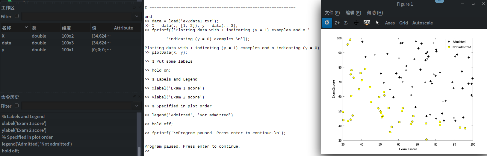
图中用+与O分别表示y = 1 与y = 0的两种结果。

在接触到真正的代价函数之前，我们通常假设函数是hΘ(x）= g（ΘTx）

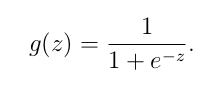
是一S形函数，他可以很好的将0与1区分开。

S形函数的实现：

function g = sigmoid(z)
%SIGMOID Compute sigmoid functoon
%   J = SIGMOID(z) computes the sigmoid of z.

% You need to return the following variables correctly
g = zeros(size(z));

% ====================== YOUR CODE HERE ======================
% Instructions: Compute the sigmoid of each value of z (z can be a matrix,
%               vector or scalar).
g = 1 ./ ( 1 + exp(-z) ) ;
% =============================================================

end

　　

现在我们可以对逻辑函数进行梯度下降，回归函数中的代价函数J(Θ)

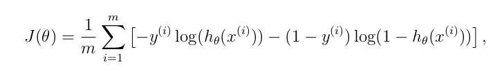
代价函数代码实现为

function [J, grad] = costFunction(theta, X, y)
%COSTFUNCTION Compute cost and gradient for logistic regression
%   J = COSTFUNCTION(theta, X, y) computes the cost of using theta as the
%   parameter for logistic regression and the gradient of the cost
%   w.r.t. to the parameters.

% Initialize some useful values
m = length(y); % number of training examples

% You need to return the following variables correctly
J = 0;
grad = zeros(size(theta));

% ====================== YOUR CODE HERE ======================
% Instructions: Compute the cost of a particular choice of theta.
%               You should set J to the cost.
%               Compute the partial derivatives and set grad to the partial
%               derivatives of the cost w.r.t. each parameter in theta
%
% Note: grad should have the same dimensions as theta
%

J= -1 * sum( y .* log( sigmoid(X*theta) ) + (1 - y ) .* log( (1 - sigmoid(X*theta)) ) ) / m ;

grad = ( X' * (sigmoid(X*theta) - y ) )/ m ;

% =============================================================

end

function [J, grad] = costFunctionReg(theta, X, y, lambda)
%COSTFUNCTIONREG Compute cost and gradient for logistic regression with regularization
%   J = COSTFUNCTIONREG(theta, X, y, lambda) computes the cost of using
%   theta as the parameter for regularized logistic regression and the
%   gradient of the cost w.r.t. to the parameters. 

% Initialize some useful values
m = length(y); % number of training examples

% You need to return the following variables correctly
J = 0;
grad = zeros(size(theta));

% ====================== YOUR CODE HERE ======================
% Instructions: Compute the cost of a particular choice of theta.
%               You should set J to the cost.
%               Compute the partial derivatives and set grad to the partial
%               derivatives of the cost w.r.t. each parameter in theta

theta_1=[0;theta(2:end)];
J= -1 * sum( y .* log( sigmoid(X*theta) ) + (1 - y ) .* log( (1 - sigmoid(X*theta)) ) ) / m  + lambda/(2*m) * theta_1' * theta_1 ;
grad = ( X' * (sigmoid(X*theta) - y ) )/ m + lambda/m * theta_1 ;

% =============================================================

end

　　

　

预测函数：

function p = predict(theta, X)
%PREDICT Predict whether the label is 0 or 1 using learned logistic
%regression parameters theta
%   p = PREDICT(theta, X) computes the predictions for X using a
%   threshold at 0.5 (i.e., if sigmoid(theta'*x) >= 0.5, predict 1)

m = size(X, 1); % Number of training examples

% You need to return the following variables correctly
p = zeros(m, 1);

% ====================== YOUR CODE HERE ======================
% Instructions: Complete the following code to make predictions using
%               your learned logistic regression parameters.
%               You should set p to a vector of 0's and 1's
%

k = find(sigmoid( X * theta) >= 0.5 );
p(k)= 1;

% p(sigmoid( X * theta) >= 0.5) = 1;   % it's a more compat way.

% =========================================================================

end

　　

　

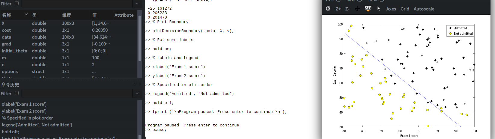
现在我们实现代价函数和他的梯度下降，并拟合出直线

%% ============ Part 2: Compute Cost and Gradient ============
%  In this part of the exercise, you will implement the cost and gradient
%  for logistic regression. You neeed to complete the code in
%  costFunction.m

%  Setup the data matrix appropriately, and add ones for the intercept term
[m, n] = size(X);

% Add intercept term to x and X_test
X = [ones(m, 1) X];

% Initialize fitting parameters
initial_theta = zeros(n + 1, 1);

% Compute and display initial cost and gradient
[cost, grad] = costFunction(initial_theta, X, y);

fprintf('Cost at initial theta (zeros): %f\n', cost);
fprintf('Gradient at initial theta (zeros): \n');
fprintf(' %f \n', grad);

fprintf('\nProgram paused. Press enter to continue.\n');
pause;

　　

%% ============= Part 3: Optimizing using fminunc  =============
%  In this exercise, you will use a built-in function (fminunc) to find the
%  optimal parameters theta.

%  Set options for fminunc
options = optimset('GradObj', 'on', 'MaxIter', 400);

%  Run fminunc to obtain the optimal theta
%  This function will return theta and the cost
[theta, cost] = ...
	fminunc(@(t)(costFunction(t, X, y)), initial_theta, options);

% Print theta to screen
fprintf('Cost at theta found by fminunc: %f\n', cost);
fprintf('theta: \n');
fprintf(' %f \n', theta);

% Plot Boundary
plotDecisionBoundary(theta, X, y);

% Put some labels
hold on;
% Labels and Legend
xlabel('Exam 1 score')
ylabel('Exam 2 score')

% Specified in plot order
legend('Admitted', 'Not admitted')
hold off;

fprintf('\nProgram paused. Press enter to continue.\n');
pause;

%% ============== Part 4: Predict and Accuracies ==============
%  After learning the parameters, you'll like to use it to predict the outcomes
%  on unseen data. In this part, you will use the logistic regression model
%  to predict the probability that a student with score 45 on exam 1 and
%  score 85 on exam 2 will be admitted.
%
%  Furthermore, you will compute the training and test set accuracies of
%  our model.
%
%  Your task is to complete the code in predict.m

%  Predict probability for a student with score 45 on exam 1
%  and score 85 on exam 2 

prob = sigmoid([1 45 85] * theta);
fprintf(['For a student with scores 45 and 85, we predict an admission ' ...
         'probability of %f\n\n'], prob);

% Compute accuracy on our training set
p = predict(theta, X);

fprintf('Train Accuracy: %f\n', mean(double(p == y)) * 100);

fprintf('\nProgram paused. Press enter to continue.\n');
pause;

　　

实例2，对非线性函数进行逻辑回归，

实现步骤如下：

%% Machine Learning Online Class - Exercise 2: Logistic Regression
%
%  Instructions
%  ------------
%
%  This file contains code that helps you get started on the second part
%  of the exercise which covers regularization with logistic regression.
%
%  You will need to complete the following functions in this exericse:
%
%     sigmoid.m
%     costFunction.m
%     predict.m
%     costFunctionReg.m
%
%  For this exercise, you will not need to change any code in this file,
%  or any other files other than those mentioned above.
%

%% Initialization
clear ; close all; clc

%% Load Data
%  The first two columns contains the X values and the third column
%  contains the label (y).

data = load('ex2data2.txt');
X = data(:, [1, 2]); y = data(:, 3);

plotData(X, y);

% Put some labels
hold on;

% Labels and Legend
xlabel('Microchip Test 1')
ylabel('Microchip Test 2')

% Specified in plot order
legend('y = 1', 'y = 0')
hold off;

%% =========== Part 1: Regularized Logistic Regression ============
%  In this part, you are given a dataset with data points that are not
%  linearly separable. However, you would still like to use logistic
%  regression to classify the data points.
%
%  To do so, you introduce more features to use -- in particular, you add
%  polynomial features to our data matrix (similar to polynomial
%  regression).
%

% Add Polynomial Features

% Note that mapFeature also adds a column of ones for us, so the intercept
% term is handled
X = mapFeature(X(:,1), X(:,2));

% Initialize fitting parameters
initial_theta = zeros(size(X, 2), 1);

% Set regularization parameter lambda to 1
lambda = 1;

% Compute and display initial cost and gradient for regularized logistic
% regression
[cost, grad] = costFunctionReg(initial_theta, X, y, lambda);

fprintf('Cost at initial theta (zeros): %f\n', cost);

fprintf('\nProgram paused. Press enter to continue.\n');
pause;

%% ============= Part 2: Regularization and Accuracies =============
%  Optional Exercise:
%  In this part, you will get to try different values of lambda and
%  see how regularization affects the decision coundart
%
%  Try the following values of lambda (0, 1, 10, 100).
%
%  How does the decision boundary change when you vary lambda? How does
%  the training set accuracy vary?
%

% Initialize fitting parameters
initial_theta = zeros(size(X, 2), 1);

% Set regularization parameter lambda to 1 (you should vary this)
lambda = 1;

% Set Options
options = optimset('GradObj', 'on', 'MaxIter', 400);

% Optimize
[theta, J, exit_flag] = ...
	fminunc(@(t)(costFunctionReg(t, X, y, lambda)), initial_theta, options);

% Plot Boundary
plotDecisionBoundary(theta, X, y);
hold on;
title(sprintf('lambda = %g', lambda))

% Labels and Legend
xlabel('Microchip Test 1')
ylabel('Microchip Test 2')

legend('y = 1', 'y = 0', 'Decision boundary')
hold off;

% Compute accuracy on our training set
p = predict(theta, X);

fprintf('Train Accuracy: %f\n', mean(double(p == y)) * 100);

　　样本：

逻辑回归：

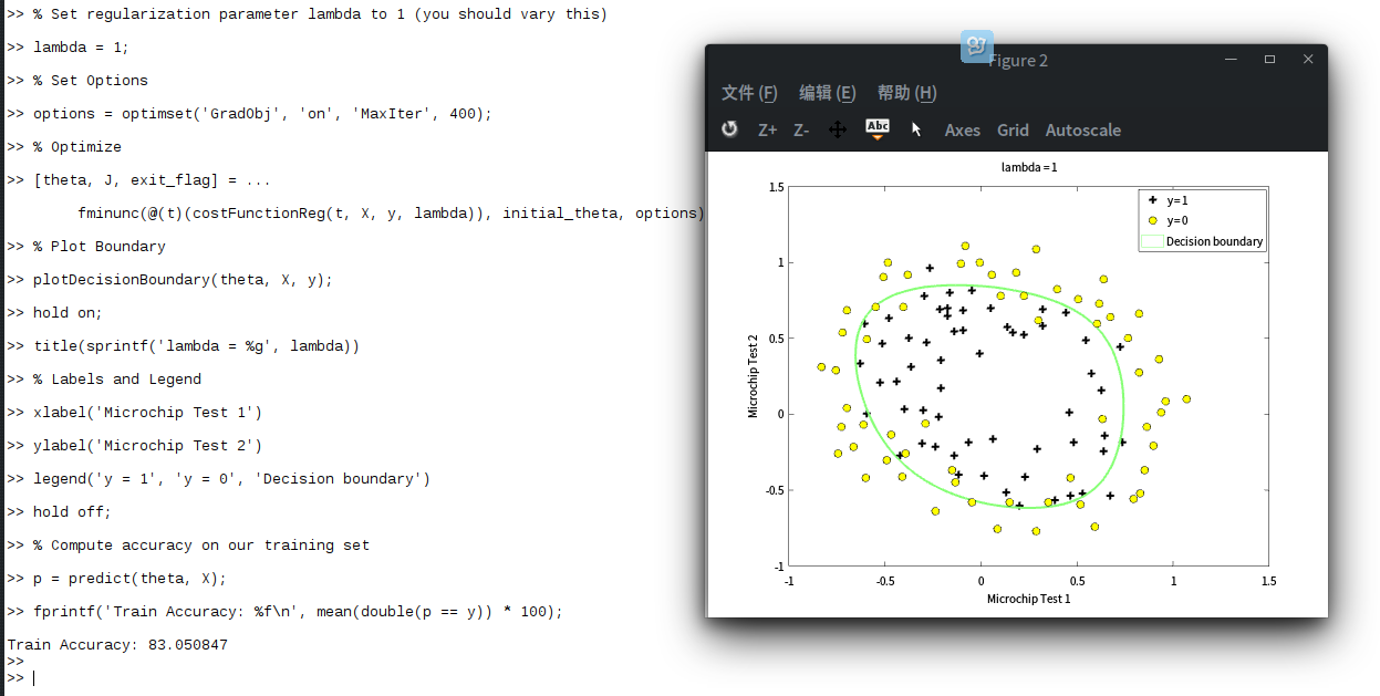
预测结果：为83.050847