[Bayes] Understanding Bayes: Updating priors via the likelihood

From: https://alexanderetz.com/2015/07/25/understanding-bayes-updating-priors-via-the-likelihood/

Reading note.

---

In a previous post I outlined the basic idea behind likelihoods and likelihood ratios. Likelihoods are relatively straightforward to understand because they are based on tangible data.

Collect your data, and then the likelihood curve shows the relative support that your data lend to various simple hypotheses.

Likelihoods are a key component of Bayesian inference because they are the bridge that gets us from prior to posterior.

In this post I explain how to use the likelihood to update a prior into a posterior. 如何 通过 似然函数 来更新 先验 --> 后验。

The simplest way to illustrate likelihoods as an updating factor is to use conjugate distribution families (Raiffa & Schlaifer, 1961). A prior and likelihood are said to be conjugate when the resulting posterior distribution is the same type of distribution as the prior. This means that

if you have binomial data you can use a beta prior to obtain a beta posterior.

If you had normal data you could use a normal prior and obtain a normal posterior.

Conjugate priors are not required for doing bayesian updating, but they make the calculations a lot easier so they are nice to use if you can.

只是说了采用共轭先验的好处。

I’ll use some data from a recent NCAA 3-point shooting contest to illustrate how different priors can converge into highly similar posteriors.

The data

This year’s NCAA shooting contest was a thriller that saw Cassandra Brown of the Portland Pilots win the grand prize. This means that she won the women’s contest and went on to defeat the men’s champion in a shoot-off.

This got me thinking, just how good is Cassandra Brown?

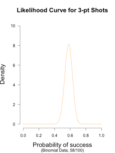
What a great chance to use some real data in a toy example. She completed 4 rounds of shooting, with 25 shots in each round, for a total of 100 shots (I did the math). The data are counts, so I’ll be using the binomial distribution as a data model (i.e., the likelihood. See this previous post for details). Her results were the following:

Round 1: 13/25               Round 2: 12/25               Round 3: 14/25               Round 4: 19/25

Total: 58/100

bin分布的样子

The likelihood curve below encompasses the entirety of statistical evidence that our 3-point data provide (footnote 1). The hypothesis with the most relative support is .58, and the curve is moderately narrow since there are quite a few data points. I didn’t standardize the height of the curve in order to keep it comparable to the other curves I’ll be showing.

The prior

Now the part that people often make a fuss about: choosing the prior. There are a few ways to choose a prior. Since I am using a binomial likelihood, I’ll be using a conjugate beta prior.

A beta prior has two shape parameters that determine what it looks like, and is denoted Beta(α, β). I like to think of priors in terms of what kind of information they represent.

The shape parameters α and β can be thought of as prior observations that I’ve made (or imagined).

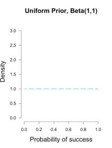
Imagine my trusted friend caught the end of Brown’s warm-up and saw her take two shots, making one and missing the other, and she tells me this information. 阶段性得知：打中一个，漏掉一个。

(1)

This would mean I could reasonably use the common Beta(1, 1) prior, which represents a uniform density over [0, 1].

In other words, all possible values for Brown’s shooting percentage are given equal weight before taking data into account, because the only thing I know about her ability is that both outcomes are possible (Lee & Wagenmakers, 2005).

(2)

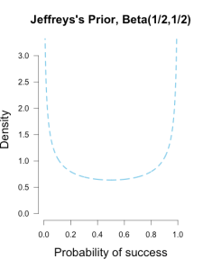
Another common prior is called Jeffreys’s prior, a Beta(1/2, 1/2) which forms a wide bowl shape.

This prior would be recommended if you had extremely scarce information about Brown’s ability. Is Brown so good that she makes nearly every shot, or is she so bad that she misses nearly every shot? This prior says that Brown’s shooting rate is probably near the extremes, which may not necessarily reflect a reasonable belief for someone who is a college basketball player, but it has the benefit of having less influence on the posterior estimates than the uniform prior (since it is equal to 1 prior observation instead of 2). Jeffreys’s prior is popular because it has some desirable properties, such as invariance under parameter transformation (Jaynes, 2003). So if instead of asking about Brown’s shooting percentage I instead wanted to know her shooting percentage squared or cubed, Jeffreys’s prior would remain the same shape while many other priors would drastically change shape.

(3)

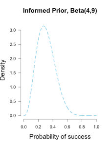
Or perhaps I had another trusted friend who had arrived earlier and seen Brown take her final 13 shots in warm-up, and she saw 4 makes and 9 misses. Then I could use a Beta(4, 9) prior to characterize this prior information, which looks like a hump over .3 with density falling slowly as it moves outward in either direction. This prior has information equivalent to 13 shots, or roughly an extra 1/2 round of shooting.

These three different priors are shown below.

  

以上就简单得举了先验例子而已，没啥干货。

These are but three possible priors one could use. In your analysis you can use any prior you want, but if you want to be taken seriously you’d better give some justification for it. Bayesian inference allows many rules for prior construction.”This is my personal prior” is a technically a valid reason, but if this is your only justification then your colleagues/reviewers/editors will probably not take your results seriously. 先验的选择至少要有一定的理由。

Now for the easiest part. In order to obtain a posterior, simply use Bayes’s rule:

The posterior is proportional to the likelihood multiplied by the prior. What’s nice about working with conjugate distributions is that Bayesian updating really is as simple as basic algebra. We take the formula for the binomial likelihood, which from a previous post is known to be:

and then multiply it by the formula for the beta prior with α and β shape parameters:

to obtain the following formula for the posterior:

With a little bit of algebra knowledge, you’ll know that multiplying together terms with the same base means the exponents can be added together. So the posterior formula can be rewritten as:

and then by adding the exponents together the formula simplifies to:

and it’s that simple! Take the prior, add the successes and failures to the different exponents, and voila. The distributional notation is even simpler. Take the prior, Beta(α, β), and add the successes from the data, x, to α and the failures, n – x, to β, and there’s your posterior, Beta(α+x, β+n-x).

Remember from the previous post that likelihoods don’t care about what order the data arrive in, it always results in the same curve. This property of likelihoods is carried over to posterior updating. The formulas above serve as another illustration of this fact. It doesn’t matter if you add a string of six single data points, 1+1+1+1+1+1+1 or a batch of +6 data points; the posterior formula in either case ends up with 6 additional points in the exponents.

以上内容可略。

Looking at some posteriors

Back to Brown’s shooting data. She had four rounds of shooting so I’ll treat each round as a batch of new data. Her results for each round were: 13/25, 12/25, 14/25, 19/25.

I’ll show how the different priors are updated with each batch of data. 先验如何被更新。

A neat thing about bayesian updating is that after batch 1 is added to the initial prior, its posterior is used as the prior for the next batch of data. 后验变为预测下一轮的先验，这里有四轮。

And as the formulas above indicate, the order or frequency of additions doesn’t make a difference on the final posterior. I’ll verify this at the end of the post.

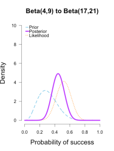
In the following plots, the prior is shown in blue (as above), the likelihood in orange (as above), and the resulting posteriors after Brown’s first 13/25 makes in purple.

  

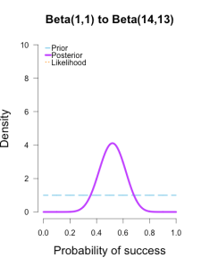
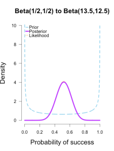
In the first and second plot the likelihood is nearly invisible because the posterior sits right on top of it. 似然被后验遮盖住了。

When the prior has only 1 or 2 data points worth of information, it has essentially no impact on the posterior shape (footnote 2).

The third plot shows how the posterior splits the difference between the likelihood and the informed prior based on the relative quantity of information in each.

The posteriors obtained from the uniform and Jeffreys’s priors suggest the best guess for Brown’s shooting percentage is around 50%, whereas the posterior obtained from the informed prior suggests it is around 40%.

No surprise here since the informed prior represents another 1/2 round of shots where Brown performed poorly, which shifts the posterior towards lower values. But all three posteriors are still quite broad, and the breadth of the curves can be thought to represent the uncertainty in my estimates. More data -> tighter curves -> less uncertainty.

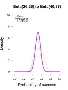
Now I’ll add the second round performance as a new likelihood (12/25 makes), and I’ll take the posteriors from the first round of updating as new priors for the second round of updating. So the purple posteriors from the plots above are now blue priors, the likelihood is orange again, and the new posteriors are purple.

  

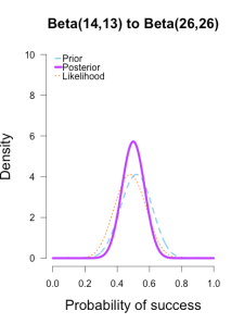
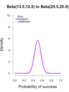
The left two plots look nearly identical, which should be no surprise since their posteriors were essentially equivalent after only 1 round of data updates. 毕竟第一轮的结果本来就很接近。

The third plot shows a posterior still slightly shifted to the left of the others, but it is much more in line with them than before. 三个曲线接近了许多。

All three posteriors are getting narrower as more data is added.

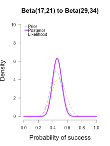
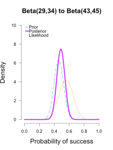
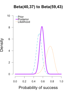
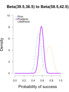
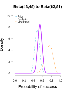
The last two rounds of updating are shown below, again with posteriors from the previous round taken as priors for the next round.

At this point they’ve all converged to very similar posteriors that are much narrower, translating to less uncertainty in my estimates.

(14/25, 19/25)

  

  

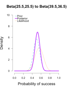
These posterior distributions look pretty similar now! Just as an illustration, 三个后验相似了许多。似然表示了当前batch的值代表的最好的sita。

I’ll show what happens when I update the initial priors with all of the data at once.

  

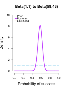
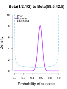
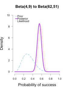
As the formulas predict, the posteriors after one big batch of data are identical to those obtained by repeatedly adding multiple smaller batches of data.

It’s also a little easier to see the discrepancies between the final posteriors in this illustration because the likelihood curve acts as a visual anchor. The uniform and Jeffreys’s priors result in posteriors that essentially fall right on top of the likelihood, whereas the informed prior results in a posterior that is very slightly shifted to the left of the likelihood.

My takeaway from these posteriors is that Cassandra Brown has a pretty damn good 3-point shot! In a future post I’ll explain how to use this method of updating to make inferences using Bayes factors.

It’s called the Savage-Dickey density method, and I think it’s incredibly intuitive and easy to use.

代码可用。

shotData<- c(1, 0, 0, 0, 1, 0, 1, 0, 1, 0, 0, 0, 1, 1, 1, 0, 1, 0, 1, 1, 1, 0, 0, 1, 1, 0, 0,
             1, 1, 1, 0, 0, 1, 1, 0, 0, 0, 1, 1, 1, 0, 0, 0, 0, 1, 1, 0, 1, 1, 0, 1, 0, 0, 1,
             0, 1, 0, 1, 1, 1, 0, 1, 0, 1, 0, 0, 1, 1, 0, 1, 0, 0, 1, 1, 1, 1, 1, 1, 1, 1, 1,
             1, 1, 1, 0, 0, 1, 1, 0, 0, 1, 1, 1, 0, 1, 1, 1, 1, 1, 0)

#figure 1 from blog, likelihood curve for 58/100 shots

x = seq(.001, .999, .001) ##Set up for creating the distributions
y2 = dbeta(x, 1 + 58, 1 + 42) # data for likelihood curve, plotted as the posterior from a beta(1,1)

plot(x, y2, xlim=c(0,1), ylim=c(0, 1.25 * max(y2,1.6)), type = "l", ylab= "Density", lty = 3,
     xlab= "Probability of success", las=1, main="Likelihood Curve for 3-pt Shots", sub= "(Binomial Data, 58/100)",lwd=2,
     cex.lab=1.5, cex.main=1.5, col = "darkorange", axes=FALSE)
axis(1, at = seq(0,1,.2)) #adds custom x axis
axis(2, las=1) # custom y axis

## Function for plotting priors, likelihoods, and posteriors for binomial data
## Output consists of a plot and various statistics
## PS and PF determine the shape of the prior distribution.
## PS = prior success, PF = prior failure for beta dist.
## PS = 1, PF = 1 corresponds to uniform(0,1) and is default. If left at default, posterior will be equivalent to likelihood
## k = number of observed successes in the data, n = total trials. If left at 0 only plots the prior dist.
## null = Is there a point-null hypothesis? null = NULL leaves it out of plots and calcs
## CI = Is there a relevant X% credibility interval? .95 is recommended and standard

plot.beta <- function(PS = 1, PF = 1, k = 0, n = 0, null = NULL, CI = NULL, ymax = "auto", main = NULL) {

  x = seq(.001, .999, .001) ##Set up for creating the distributions
  y1 = dbeta(x, PS, PF) # data for prior curve
  y3 = dbeta(x, PS + k, PF + n - k) # data for posterior curve
  y2 = dbeta(x, 1 + k, 1 + n - k) # data for likelihood curve, plotted as the posterior from a beta(1,1)

  if(is.numeric(ymax) == T){ ##you can specify the y-axis maximum
    y.max = ymax
  }
  else(
    y.max = 1.25 * max(y1,y2,y3,1.6) ##or you can let it auto-select
  )

  if(is.character(main) == T){
    Title = main
  }
  else(
    Title = "Prior-to-Posterior Transformation with Binomial Data"
  )

  plot(x, y1, xlim=c(0,1), ylim=c(0, y.max), type = "l", ylab= "Density", lty = 2,
       xlab= "Probability of success", las=1, main= Title,lwd=3,
       cex.lab=1.5, cex.main=1.5, col = "skyblue", axes=FALSE)

  axis(1, at = seq(0,1,.2)) #adds custom x axis
  axis(2, las=1) # custom y axis

  if(n != 0){
    #if there is new data, plot likelihood and posterior
    lines(x, y2, type = "l", col = "darkorange", lwd = 2, lty = 3)
    lines(x, y3, type = "l", col = "darkorchid1", lwd = 5)
    legend("topleft", c("Prior", "Posterior", "Likelihood"), col = c("skyblue", "darkorchid1", "darkorange"),
           lty = c(2,1,3), lwd = c(3,5,2), bty = "n", y.intersp = .55, x.intersp = .1, seg.len=.7)

    ## adds null points on prior and posterior curve if null is specified and there is new data
    if(is.numeric(null) == T){
      ## Adds points on the distributions at the null value if there is one and if there is new data
      points(null, dbeta(null, PS, PF), pch = 21, bg = "blue", cex = 1.5)
      points(null, dbeta(null, PS + k, PF + n - k), pch = 21, bg = "darkorchid", cex = 1.5)
      abline(v=null, lty = 5, lwd = 1, col = "grey73")
      ##lines(c(null,null),c(0,1.11*max(y1,y3,1.6))) other option for null line
    }
  }

  ##Specified CI% but no null? Calc and report only CI
  if(is.numeric(CI) == T && is.numeric(null) == F){
    CI.low <- qbeta((1-CI)/2, PS + k, PF + n - k)
    CI.high <- qbeta(1-(1-CI)/2, PS + k, PF + n - k)

    SEQlow<-seq(0, CI.low, .001)
    SEQhigh <- seq(CI.high, 1, .001)
    ##Adds shaded area for x% Posterior CIs
    cord.x <- c(0, SEQlow, CI.low) ##set up for shading
    cord.y <- c(0,dbeta(SEQlow,PS + k, PF + n - k),0) ##set up for shading
    polygon(cord.x,cord.y,col='orchid', lty= 3) ##shade left tail
    cord.xx <- c(CI.high, SEQhigh,1)
    cord.yy <- c(0,dbeta(SEQhigh,PS + k, PF + n - k), 0)
    polygon(cord.xx,cord.yy,col='orchid', lty=3) ##shade right tail

    return( list( "Posterior CI lower" = round(CI.low,3), "Posterior CI upper" = round(CI.high,3)))
  }

  ##Specified null but not CI%? Calculate and report BF only
  if(is.numeric(null) == T && is.numeric(CI) == F){
    null.H0 <- dbeta(null, PS, PF)
    null.H1 <- dbeta(null, PS + k, PF + n - k)
    CI.low <- qbeta((1-CI)/2, PS + k, PF + n - k)
    CI.high <- qbeta(1-(1-CI)/2, PS + k, PF + n - k)
    return( list("BF01 (in favor of H0)" = round(null.H1/null.H0,3), "BF10 (in favor of H1)" = round(null.H0/null.H1,3)
    ))
  }

  ##Specified both null and CI%? Calculate and report both
  if(is.numeric(null) == T && is.numeric(CI) == T){
    null.H0 <- dbeta(null, PS, PF)
    null.H1 <- dbeta(null, PS + k, PF + n - k)
    CI.low <- qbeta((1-CI)/2, PS + k, PF + n - k)
    CI.high <- qbeta(1-(1-CI)/2, PS + k, PF + n - k)

    SEQlow<-seq(0, CI.low, .001)
    SEQhigh <- seq(CI.high, 1, .001)
    ##Adds shaded area for x% Posterior CIs
    cord.x <- c(0, SEQlow, CI.low) ##set up for shading
    cord.y <- c(0,dbeta(SEQlow,PS + k, PF + n - k),0) ##set up for shading
    polygon(cord.x,cord.y,col='orchid', lty= 3) ##shade left tail
    cord.xx <- c(CI.high, SEQhigh,1)
    cord.yy <- c(0,dbeta(SEQhigh,PS + k, PF + n - k), 0)
    polygon(cord.xx,cord.yy,col='orchid', lty=3) ##shade right tail

    return( list("BF01 (in favor of H0)" = round(null.H1/null.H0,3), "BF10 (in favor of H1)" = round(null.H0/null.H1,3),
                 "Posterior CI lower" = round(CI.low,3), "Posterior CI upper" = round(CI.high,3)))
  }

}

#plot dimensions (415,550) for the blog figures

#Initial Priors
plot.beta(1,1,ymax=3.2,main="Uniform Prior, Beta(1,1)")
plot.beta(.5,.5,ymax=3.2,main="Jeffreys's Prior, Beta(1/2,1/2)")
plot.beta(4,9,ymax=3.2,main="Informed Prior, Beta(4,9)")

#Posteriors after Round 1
plot.beta(1,1,13,25,main="Beta(1,1) to Beta(14,13)",ymax=10)
plot.beta(.5,.5,13,25,main="Beta(1/2,1/2) to Beta(13.5,12.5)",ymax=10)
plot.beta(4,9,13,25,main="Beta(4,9) to Beta(17,21)",ymax=10)

#Posteriors after Round 2
plot.beta(14,13,12,25,ymax=10,main="Beta(14,13) to Beta(26,26)")
plot.beta(13.5,12.5,12,25,ymax=10,main="Beta(13.5,12.5) to Beta(25.5,25.5)")
plot.beta(17,21,12,25,ymax=10,main="Beta(17,21) to Beta(29,34)")

#Posteriors after Round 3
plot.beta(26,26,14,25,ymax=10,main="Beta(26,26) to Beta(40,37)")
plot.beta(25.5,25.5,14,25,ymax=10,main="Beta(25.5,25.5) to Beta(39.5,36.5)")
plot.beta(29,34,14,25,ymax=10,main="Beta(29,34) to Beta(43,45)")

#Posteriors after Round 4
plot.beta(40,37,19,25,ymax=10,main="Beta(40,37) to Beta(59,43)")
plot.beta(39.5,36.5,19,25,ymax=10,main="Beta(39.5,36.5) to Beta(58.5,42.5)")
plot.beta(43,45,19,25,ymax=10,main="Beta(43,45) to Beta(62,51)")

#Initial Priors and final Posteriors after all rounds at once
plot.beta(1,1,58,100,ymax=10,main="Beta(1,1) to Beta(59,43)")
plot.beta(.5,.5,58,100,ymax=10,main="Beta(1/2,1/2) to Beta(58.5,42.5)")
plot.beta(4,9,58,100,ymax=10,main="Beta(4,9) to Beta(62,51)")