TensorFlow实战第四课(tensorboard数据可视化)

tensorboard可视化工具

tensorboard是tensorflow的可视化工具，通过这个工具我们可以很清楚的看到整个神经网络的结构及框架。

通过之前展示的代码，我们进行修改从而展示其神经网络结构。

一、搭建图纸

首先对input进行修改，将xs，ys进行新的名称指定x_in y_in

这里指定的名称，之后会在可视化图层中inputs中显示出来

xs= tf.placeholder(tf.float32, [None, 1],name='x_in')

ys= tf.placeholder(tf.loat32, [None, 1],name='y_in')

使用with.tf.name_scope('inputs')可以将xs  ys包含进来，形成一个大的图层，图层的名字就是

with.tf.name_scope()方法中的参数

with tf.name_scope('inputs'):
    # define placeholder for inputs to network
    xs = tf.placeholder(tf.float32, [None, 1])
    ys = tf.placeholder(tf.float32, [None, 1])

接下来编辑layer

编辑前的代码片段：

def add_layer(inputs, in_size, out_size, activation_function=None):
    # add one more layer and return the output of this layer
    Weights = tf.Variable(tf.random_normal([in_size, out_size]))
    biases = tf.Variable(tf.zeros([1, out_size]) + 0.1)
    Wx_plus_b = tf.add(tf.matmul(inputs, Weights), biases)
    if activation_function is None:
        outputs = Wx_plus_b
    else:
        outputs = activation_function(Wx_plus_b, )
    return outputs

编辑后

def add_layer(inputs, in_size, out_size, activation_function=None):
    # add one more layer and return the output of this layer
    with tf.name_scope('layer'):
        Weights= tf.Variable(tf.random_normal([in_size, out_size]))
        # and so on...

定义完大的框架layer后，通知需要定义里面小的部件weights biases activationfunction

定义方法有两种，一是用tf.name_scope（），二是在Weights中指定名称W

    def add_layer(inputs, in_size, out_size, activation_function=None):
    #define layer name
    with tf.name_scope('layer'):
        #define weights name
        with tf.name_scope('weights'):
            Weights= tf.Variable(tf.random_normal([in_size, out_size]),name='W')
        #and so on......

接着定义biases，方法同上

def add_layer(inputs, in_size, out_size, activation_function=None):
    #define layer name
    with tf.name_scope('layer'):
        #define weights name
        with tf.name_scope('weights')
            Weights= tf.Variable(tf.random_normal([in_size, out_size]),name='W')
        # define biase
        with tf.name_scope('Wx_plus_b'):
            Wx_plus_b = tf.add(tf.matmul(inputs, Weights), biases)
        # and so on....

最后编辑loss 将with.tf.name_scope( )添加在loss上方 并起名为loss

这句话就是绘制了loss

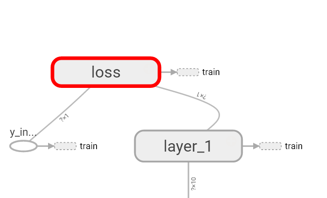
最后再对train_step进行编辑

with tf.name_scope('train'):
    train_step = tf.train.GradientDescentOptimizer(0.1).minimize(loss)

我们还需要运用tf.summary.FileWriter( )将上面绘画的图保存到一个目录中，方便用浏览器浏览。

这个方法中的第二个参数需要使用sess.graph。因此我们把这句话放在获取session后面。

这里的graph是将前面定义的框架信息收集起来，然后放在logs/目录下面。

sess = tf.Session() # get session
# tf.train.SummaryWriter soon be deprecated, use following
writer = tf.summary.FileWriter("logs/", sess.graph)

最后在终端中使用命令获取网址即可查看

tensorboard --logdir logs

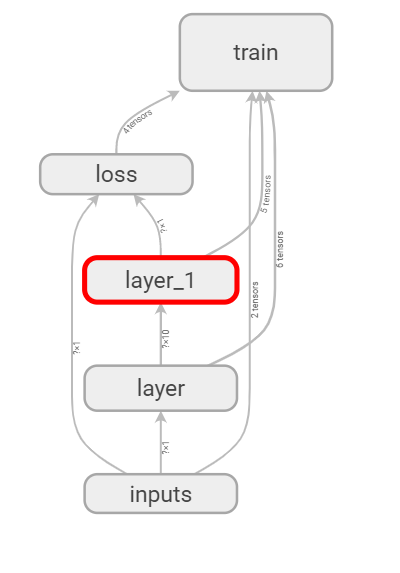
完整代码：

#如何可视化神经网络

#tensorboard

import tensorflow as tf

def add_layer(inputs, in_size, out_size, activation_function=None):
    # add one more layer and return the output of this layer
    with tf.name_scope('layer'):
        with tf.name_scope('weights'):
            Weights = tf.Variable(tf.random_normal([in_size, out_size]), name='W')
        with tf.name_scope('biases'):
            biases = tf.Variable(tf.zeros([1, out_size]) + 0.1, name='b')
        with tf.name_scope('Wx_plus_b'):
            Wx_plus_b = tf.add(tf.matmul(inputs, Weights), biases)
        if activation_function is None:
            outputs = Wx_plus_b
        else:
            outputs = activation_function(Wx_plus_b)
        return outputs

# define placeholder for inputs to network
with tf.name_scope('inputs'):
    xs = tf.placeholder(tf.float32, [None, 1], name='x_input')
    ys = tf.placeholder(tf.float32, [None, 1], name='y_input')

# add hidden layer
l1 = add_layer(xs, 1, 10, activation_function=tf.nn.relu)
# add output layer
prediction = add_layer(l1, 10, 1, activation_function=None)

# the error between prediciton and real data
with tf.name_scope('loss'):
    loss = tf.reduce_mean(tf.reduce_sum(tf.square(ys - prediction), reduction_indices=[1]))

with tf.name_scope('train'):
    train_step = tf.train.GradientDescentOptimizer(0.1).minimize(loss)

sess = tf.Session()

writer = tf.summary.FileWriter("logs/", sess.graph)

init = tf.global_variables_initializer()

sess.run(init)

-------------------------------------------------------------------

tensorflow可视化训练过程的图标是如何制作的？

首先要添加一些模拟数据。nump可以帮助我们添加一些模拟数据。

利用np.linespace（）产生随机的数字 同时为了模拟更加真实 我们会添加一些噪声 这些噪声是通过np.random.normal（）随机产生的。

 x_data= np.linspace(-1, 1, 300, dtype=np.float32)[:,np.newaxis]
 noise=  np.random.normal(0, 0.05, x_data.shape).astype(np.float32)
 y_data= np.square(x_data) -0.5+ noise

在layer中为weights biases设置变化图表

首先我们在add_layer（）方法中添加一个参数n_layer 来标识层数 并且用变量layer_name代表其每层的名称

def add_layer(
    inputs ,
    in_size,
    out_size,
    n_layer,
    activation_function=None):
    ## add one more layer and return the output of this layer
    layer_name='layer%s'%n_layer  ## 定义一个新的变量
    ## and so on ……

接下来 我们层中的Weights设置变化图 tensorflow中提供了tf.histogram_summary( )方法，用来绘制图片，第一个参数是图表的名称，第二个参数是图标要记录的变量。

def add_layer(inputs ,
            in_size,
            out_size,n_layer,
            activation_function=None):
    ## add one more layer and return the output of this layer
    layer_name='layer%s'%n_layer
    with tf.name_scope('layer'):
         with tf.name_scope('weights'):
              Weights= tf.Variable(tf.random_normal([in_size, out_size]),name='W')
              tf.summary.histogram(layer_name + '/weights', Weights)
    ##and so no ……

同样的方法我们对biases进行绘制图标：

with tf.name_scope('biases'):
    biases = tf.Variable(tf.zeros([1,out_size])+0.1, name='b')
    tf.summary.histogram(layer_name + '/biases', biases)  

至于activation_function( ) 可以不用绘制，我们对output 使用同样的方法

最后通过修改 addlayer（）方法如下所示

def add_layer(inputs, in_size, out_size, n_layer, activation_function=None):
    # add one more layer and return the output of this layer

    #对神经层进行命名
    layer_name = 'layer%s' % n_layer
    with tf.name_scope(layer_name):
        with tf.name_scope('weights'):
            Weights = tf.Variable(tf.random_normal([in_size, out_size]), name='W')
            tf.summary.histogram(layer_name + '/weights', Weights)
        with tf.name_scope('biases'):
            biases = tf.Variable(tf.zeros([1, out_size]) + 0.1, name='b')
            tf.summary.histogram(layer_name + '/biases', biases)
        with tf.name_scope('Wx_plus_b'):
            Wx_plus_b = tf.add(tf.matmul(inputs, Weights), biases)
        if activation_function is None:
            outputs = Wx_plus_b
        else:
            outputs = activation_function(Wx_plus_b, )
        tf.summary.histogram(layer_name + '/outputs', outputs)
    return outputs

设置loss的变化图

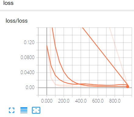
loss是tensorb的event下面的 这是由于我们使用的是tf.scalar_summary（）方法。

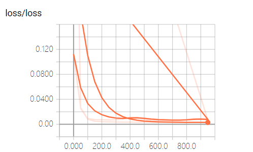
当你的loss函数图像呈现的是下降的趋势 说明学习是有效的

将所有训练图合并

接下来进行合并打包，tf.merge_all_summaries（）方法会对我们所有的summaries合并到一起

sess = tf.Session()
#合并
merged = tf.summary.merge_all()

writer = tf.summary.FileWriter("logs/", sess.graph)

init = tf.global_variables_initializer()

训练数据

忽略不想写

完整代码如下：（运行代码后需要在终端中执行tensorboard --logdir logs）

import tensorflow as tf
import numpy as np

def add_layer(inputs, in_size, out_size, n_layer, activation_function=None):
    # add one more layer and return the output of this layer

    #对神经层进行命名
    layer_name = 'layer%s' % n_layer
    with tf.name_scope(layer_name):
        with tf.name_scope('weights'):
            Weights = tf.Variable(tf.random_normal([in_size, out_size]), name='W')
            tf.summary.histogram(layer_name + '/weights', Weights)
        with tf.name_scope('biases'):
            biases = tf.Variable(tf.zeros([1, out_size]) + 0.1, name='b')
            tf.summary.histogram(layer_name + '/biases', biases)
        with tf.name_scope('Wx_plus_b'):
            Wx_plus_b = tf.add(tf.matmul(inputs, Weights), biases)
        if activation_function is None:
            outputs = Wx_plus_b
        else:
            outputs = activation_function(Wx_plus_b, )
        tf.summary.histogram(layer_name + '/outputs', outputs)
    return outputs

# Make up some real data
x_data = np.linspace(-1, 1, 300)[:, np.newaxis]
noise = np.random.normal(0, 0.05, x_data.shape)
y_data = np.square(x_data) - 0.5 + noise

# define placeholder for inputs to network
with tf.name_scope('inputs'):
    xs = tf.placeholder(tf.float32, [None, 1], name='x_input')
    ys = tf.placeholder(tf.float32, [None, 1], name='y_input')

# add hidden layer
l1 = add_layer(xs, 1, 10, n_layer=1, activation_function=tf.nn.relu)
# add output layer
prediction = add_layer(l1, 10, 1, n_layer=2, activation_function=None)

# the error between prediciton and real data
with tf.name_scope('loss'):
    loss = tf.reduce_mean(tf.reduce_sum(tf.square(ys - prediction),
                                        reduction_indices=[1]))
    tf.summary.scalar('loss', loss)

with tf.name_scope('train'):
    train_step = tf.train.GradientDescentOptimizer(0.1).minimize(loss)

sess = tf.Session()
#合并
merged = tf.summary.merge_all()

writer = tf.summary.FileWriter("logs/", sess.graph)

init = tf.global_variables_initializer()
sess.run(init)

for i in range(1000):
    sess.run(train_step, feed_dict={xs: x_data, ys: y_data})
    if i % 50 == 0:
        result = sess.run(merged,feed_dict={xs: x_data, ys: y_data})
        #i 就是记录的步数
        writer.add_summary(result, i)

tensorboard查看效果  使用命令tensorboard --logdir logs