课程四(Convolutional Neural Networks)，第一周（Foundations of Convolutional Neural Networks） —— 3.Programming assignments：Convolutional Model: application

Convolutional Neural Networks: Application

Welcome to Course 4's second assignment! In this notebook, you will:

• Implement helper functions that you will use when implementing a TensorFlow model
• Implement a fully functioning ConvNet using TensorFlow (使用 TensorFlow 实现完全正常运行的 ConvNet)

After this assignment you will be able to:

• Build and train a ConvNet in TensorFlow for a classification problem

We assume here that you are already familiar with TensorFlow. If you are not, please refer the TensorFlow Tutorial of the third week of Course 2 ("Improving deep neural networks").

1.0 - TensorFlow model

In the previous assignment, you built helper functions using numpy to understand the mechanics behind convolutional neural networks. Most practical applications of deep learning today are built using programming frameworks, which have many built-in functions you can simply call.

As usual, we will start by loading in the packages.

【code】

import math
import numpy as np
import h5py
import matplotlib.pyplot as plt
import scipy
from PIL import Image
from scipy import ndimage
import tensorflow as tf
from tensorflow.python.framework import ops
from cnn_utils import *

%matplotlib inline
np.random.seed(1)

Run the next cell to load the "SIGNS" dataset you are going to use.

【code】

# Loading the data (signs)
X_train_orig, Y_train_orig, X_test_orig, Y_test_orig, classes = load_dataset()

As a reminder, the SIGNS dataset is a collection of 6 signs representing numbers from 0 to 5.

The next cell will show you an example of a labelled image in the dataset. Feel free to change the value of index below and re-run to see different examples.

【code】

# Example of a picture
index = 6
plt.imshow(X_train_orig[index])
print ("y = " + str(np.squeeze(Y_train_orig[:, index])))

【result】

y = 2

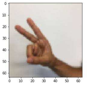
In Course 2, you had built a fully-connected network for this dataset. But since this is an image dataset, it is more natural to apply a ConvNet to it.

To get started, let's examine the shapes of your data.

【code】

X_train = X_train_orig/255.
X_test = X_test_orig/255.
Y_train = convert_to_one_hot(Y_train_orig, 6).T    #convert_to_one_hot(Y, C)函数参见课程二第三周的2、programming assignments: 1.4 Using One Hot Encodeings
Y_test = convert_to_one_hot(Y_test_orig, 6).T
print ("number of training examples = " + str(X_train.shape[0]))
print ("number of test examples = " + str(X_test.shape[0]))
print ("X_train shape: " + str(X_train.shape))
print ("Y_train shape: " + str(Y_train.shape))
print ("X_test shape: " + str(X_test.shape))
print ("Y_test shape: " + str(Y_test.shape))
conv_layers = {}

【result】

number of training examples = 1080
number of test examples = 120
X_train shape: (1080, 64, 64, 3)
Y_train shape: (1080, 6)
X_test shape: (120, 64, 64, 3)
Y_test shape: (120, 6)

1.1 - Create placeholders

TensorFlow requires that you create placeholders for the input data that will be fed into the model when running the session.

Exercise: Implement the function below to create placeholders for the input image X and the output Y. You should not define the number of training examples for the moment. To do so, you could use "None" as the batch size, it will give you the flexibility to choose it later. Hence X should be of dimension [None, n_H0, n_W0, n_C0] and Y should be of dimension [None, n_y]. Hint.   （参见课程二第三周的2、programming assignments: 2.1 Create placeholders)

【code】

# GRADED FUNCTION: create_placeholders

def create_placeholders(n_H0, n_W0, n_C0, n_y):     #参见课程二第三周的2、programming assignments: 2.1 Create placeholders
    """
    Creates the placeholders for the tensorflow session.

    Arguments:
    n_H0 -- scalar, height of an input image
    n_W0 -- scalar, width of an input image
    n_C0 -- scalar, number of channels of the input
    n_y -- scalar, number of classes

    Returns:
    X -- placeholder for the data input, of shape [None, n_H0, n_W0, n_C0] and dtype "float"
    Y -- placeholder for the input labels, of shape [None, n_y] and dtype "float"
    """

    ### START CODE HERE ### (≈2 lines)
    X = tf.placeholder(dtype=tf.float32,shape=[None, n_H0, n_W0, n_C0], name = "Placeholder")
    Y =  tf.placeholder(dtype=tf.float32,shape=[None, n_y], name = "Placeholder_1")
    ### END CODE HERE ###

    return X, Y

X, Y = create_placeholders(64, 64, 3, 6)
print ("X = " + str(X))
print ("Y = " + str(Y))

【result】

X = Tensor("Placeholder:0", shape=(?, 64, 64, 3), dtype=float32)
Y = Tensor("Placeholder_1:0", shape=(?, 6), dtype=float32)

Expected Output:

X = Tensor("Placeholder:0", shape=(?, 64, 64, 3), dtype=float32)
Y = Tensor("Placeholder_1:0", shape=(?, 6), dtype=float32)

1.2 - Initialize parameters

You will initialize weights/filters W1W1 and W2W2 using tf.contrib.layers.xavier_initializer(seed = 0). You don't need to worry about bias variables as you will soon see that TensorFlow functions take care of the bias. Note also that you will only initialize the weights/filters for the conv2d functions. TensorFlow initializes the layers for the fully connected part automatically. We will talk more about that later in this assignment.

Exercise: Implement initialize_parameters(). The dimensions for each group of filters are provided below. Reminder - to initialize a parameter WW of shape [1,2,3,4] in Tensorflow, use:

 

W = tf.get_variable("W", [1,2,3,4], initializer = ...)

More Info.

【code】

tf.reset_default_graph()  # ？？
with tf.Session() as sess_test:
    parameters = initialize_parameters()
    init = tf.global_variables_initializer()
    sess_test.run(init)
    print("W1 = " + str(parameters["W1"].eval()[1,1,1]))   # ??
    print("W2 = " + str(parameters["W2"].eval()[1,1,1]))   # ??

【result】

W1 = [ 0.00131723  0.14176141 -0.04434952  0.09197326  0.14984085 -0.03514394
 -0.06847463  0.05245192]
W2 = [-0.08566415  0.17750949  0.11974221  0.16773748 -0.0830943  -0.08058
 -0.00577033 -0.14643836  0.24162132 -0.05857408 -0.19055021  0.1345228
 -0.22779644 -0.1601823  -0.16117483 -0.10286498]

Expected Output:

W1 =    [ 0.00131723 0.14176141 -0.04434952 0.09197326 0.14984085 -0.03514394
-0.06847463 0.05245192]
W2 =    [-0.08566415 0.17750949 0.11974221 0.16773748 -0.0830943 -0.08058
-0.00577033 -0.14643836 0.24162132 -0.05857408 -0.19055021 0.1345228
-0.22779644 -0.1601823 -0.16117483 -0.10286498]

1.2 - Forward propagation

In TensorFlow, there are built-in functions that carry out the convolution steps for you.

• tf.nn.conv2d(X,W1, strides = [1,s,s,1], padding = 'SAME'): given an input X and a group of filters W1, this function convolves W1's filters on X. The third input ([1,s,s,1]) represents the strides for each dimension of the input (m, n_H_prev, n_W_prev, n_C_prev). You can read the full documentation here

• tf.nn.max_pool(A, ksize = [1,f,f,1], strides = [1,s,s,1], padding = 'SAME'): given an input A, this function uses a window of size (f, f) and strides of size (s, s) to carry out max pooling over each window. You can read the full documentation here

• tf.nn.relu(Z1): computes the elementwise ReLU of Z1 (which can be any shape). You can read the full documentation here.

• tf.contrib.layers.flatten(P): given an input P, this function flattens each example into a 1D vector it while maintaining the batch-size. It returns a flattened tensor with shape [batch_size, k]. You can read the full documentation here.

• tf.contrib.layers.fully_connected(F, num_outputs): given a the flattened input F, it returns the output computed using a fully connected layer. You can read the full documentation here.

In the last function above (tf.contrib.layers.fully_connected), the fully connected layer automatically initializes weights in the graph and keeps on training them as you train the model. Hence, you did not need to initialize those weights when initializing the parameters.

 

Exercise:

Implement the forward_propagation function below to build the following model: CONV2D -> RELU -> MAXPOOL -> CONV2D -> RELU -> MAXPOOL -> FLATTEN -> FULLYCONNECTED. You should use the functions above.

In detail, we will use the following parameters for all the steps:

 - Conv2D: stride 1, padding is "SAME"
 - ReLU
 - Max pool: Use an 8 by 8 filter size and an 8 by 8 stride, padding is "SAME"
 - Conv2D: stride 1, padding is "SAME"
 - ReLU
 - Max pool: Use a 4 by 4 filter size and a 4 by 4 stride, padding is "SAME"
 - Flatten the previous output.
 - FULLYCONNECTED (FC) layer: Apply a fully connected layer without an non-linear activation function. Do not call the softmax here. This will result in 6 neurons 
                              in the output layer, which then get passed later to a softmax. In TensorFlow, the softmax and cost function are lumped together into 
                              a single function, which you'll call in a different function when computing the cost. 

【code】

# GRADED FUNCTION: forward_propagation

def forward_propagation(X, parameters):
    """
    Implements the forward propagation for the model:
    CONV2D -> RELU -> MAXPOOL -> CONV2D -> RELU -> MAXPOOL -> FLATTEN -> FULLYCONNECTED

    Arguments:
    X -- input dataset placeholder, of shape (input size, number of examples)   # X =[None, n_H0, n_W0, n_C0]
    parameters -- python dictionary containing your parameters "W1", "W2"
                  the shapes are given in initialize_parameters

    Returns:
    Z3 -- the output of the last LINEAR unit
    """

    # Retrieve the parameters from the dictionary "parameters"
    W1 = parameters['W1']
    W2 = parameters['W2']

    ### START CODE HERE ###
    # CONV2D: stride of 1, padding 'SAME'
    Z1 = tf.nn.conv2d(X,W1, strides = [1,1,1,1], padding = 'SAME')
    # RELU
    A1 = tf.nn.relu(Z1)
    # MAXPOOL: window 8x8, sride 8, padding 'SAME'
    P1 = tf.nn.max_pool(A1, ksize = [1,8,8,1], strides = [1,8,8,1], padding = 'SAME')
    # CONV2D: filters W2, stride 1, padding 'SAME'
    Z2 =  tf.nn.conv2d(P1,W2, strides = [1,1,1,1], padding = 'SAME')
    # RELU
    A2 = tf.nn.relu(Z2)
    # MAXPOOL: window 4x4, stride 4, padding 'SAME'
    P2 =  tf.nn.max_pool(A2, ksize = [1,4,4,1], strides = [1,4,4,1], padding = 'SAME')
    # FLATTEN
    P2 = tf.contrib.layers.flatten(P2)
    # FULLY-CONNECTED without non-linear activation function (not not call softmax).
    # 6 neurons in output layer. Hint: one of the arguments should be "activation_fn=None"
    Z3 = tf.contrib.layers.fully_connected(P2, 6,activation_fn=None)
    ### END CODE HERE ###

    return Z3

tf.reset_default_graph()

with tf.Session() as sess:
    np.random.seed(1)
    X, Y = create_placeholders(64, 64, 3, 6)
    parameters = initialize_parameters()
    Z3 = forward_propagation(X, parameters)
    init = tf.global_variables_initializer()
    sess.run(init)
    a = sess.run(Z3, {X: np.random.randn(2,64,64,3), Y: np.random.randn(2,6)})
    print("Z3 = " + str(a))
    # print(a.shape)  (2,6)

【result】

Z3 = [[-0.44670227 -1.57208765 -1.53049231 -2.31013036 -1.29104376  0.46852064]
      [-0.17601591 -1.57972014 -1.4737016  -2.61672091 -1.00810647  0.5747785 ]]

Expected Output:

Z3 =    [[-0.44670227 -1.57208765 -1.53049231 -2.31013036 -1.29104376 0.46852064]
         [-0.17601591 -1.57972014 -1.4737016  -2.61672091 -1.00810647 0.5747785 ]]

1.3 - Compute cost

Implement the compute cost function below. You might find these two functions helpful:

• tf.nn.softmax_cross_entropy_with_logits(logits = Z3, labels = Y): computes the softmax entropy loss. This function both computes the softmax activation function as well as the resulting loss. You can check the full documentation here.
• tf.reduce_mean: computes the mean of elements across dimensions of a tensor(计算张量的各个维度的元素的平均值). Use this to sum the losses over all the examples to get the overall cost. You can check the full documentation here.

Exercise: Compute the cost below using the function above.

【code】

# GRADED FUNCTION: compute_cost 

def compute_cost(Z3, Y):
    """
    Computes the cost

    Arguments:
    Z3 -- output of forward propagation (output of the last LINEAR unit), of shape (6, number of examples) #此处有误，[batch_size, num_classes]
          应该为 of shape (number of examples,6)
    Y -- "true" labels vector placeholder, same shape as Z3

    Returns:
    cost - Tensor of the cost function
    """

    ### START CODE HERE ### (1 line of code)
    cost =tf.reduce_mean(tf.nn.softmax_cross_entropy_with_logits(logits = Z3, labels = Y))
    ### END CODE HERE ###

    return cost

tf.reset_default_graph()  # （1）tf.get_default_graph()：返回返回当前线程的默认图。
                          #（2）tf.reset_default_graph()：清除默认图的堆栈，并设置全局图为默认图。

with tf.Session() as sess:
    np.random.seed(1)   #使得运行结果不变
    X, Y = create_placeholders(64, 64, 3, 6)   #占位符
    parameters = initialize_parameters() # 初始化 W1，W2
    Z3 = forward_propagation(X, parameters) #前向传播
    cost = compute_cost(Z3, Y)
    init = tf.global_variables_initializer()
    sess.run(init)  # 初始化全局变量
    a = sess.run(cost, feed_dict={X: np.random.randn(4,64,64,3), Y: np.random.randn(4,6)})  #计算cost
    print("cost = " + str(a))

【result】

cost = 2.91034

Expected Output:

cost =    2.91034

1.4 Model

Finally you will merge the helper functions you implemented above to build a model. You will train it on the SIGNS dataset.

You have implemented random_mini_batches() in the Optimization programming assignment of course 2. Remember that this function returns a list of mini-batches.

# random_mini_batches()   2 - Mini-Batch Gradient descent 。

Exercise: Complete the function below.

The model below should:

• create placeholders
• initialize parameters
• forward propagate
• compute the cost
• create an optimizer

Finally you will create a session and run a for loop for num_epochs, get the mini-batches, and then for each mini-batch you will optimize the function. Hint for initializing the variables

【code】

# GRADED FUNCTION: model

def model(X_train, Y_train, X_test, Y_test, learning_rate = 0.009,
          num_epochs = 100, minibatch_size = 64, print_cost = True):
    """
    Implements a three-layer ConvNet in Tensorflow:
    CONV2D -> RELU -> MAXPOOL -> CONV2D -> RELU -> MAXPOOL -> FLATTEN -> FULLYCONNECTED

    Arguments:
    X_train -- training set, of shape (None, 64, 64, 3)
    Y_train -- test set, of shape (None, n_y = 6)
    X_test -- training set, of shape (None, 64, 64, 3)
    Y_test -- test set, of shape (None, n_y = 6)
    learning_rate -- learning rate of the optimization
    num_epochs -- number of epochs of the optimization loop
    minibatch_size -- size of a minibatch
    print_cost -- True to print the cost every 100 epochs

    Returns:
    train_accuracy -- real number, accuracy on the train set (X_train)
    test_accuracy -- real number, testing accuracy on the test set (X_test)
    parameters -- parameters learnt by the model. They can then be used to predict.
    """

    ops.reset_default_graph()                         # to be able to rerun the model without overwriting tf variables(能够在不覆盖 tf 变量的情况下重新运行模型)
    tf.set_random_seed(1)                             # to keep results consistent (tensorflow seed)
    seed = 3                                          # to keep results consistent (numpy seed)
    (m, n_H0, n_W0, n_C0) = X_train.shape
    n_y = Y_train.shape[1]
    costs = []                                        # To keep track of the cost

    # Create Placeholders of the correct shape
    ### START CODE HERE ### (1 line)
    X, Y = create_placeholders(n_H0, n_W0, n_C0, n_y)
    ### END CODE HERE ###

    # Initialize parameters
    ### START CODE HERE ### (1 line)
    parameters = initialize_parameters()
    ### END CODE HERE ###

    # Forward propagation: Build the forward propagation in the tensorflow graph
    ### START CODE HERE ### (1 line)
    Z3 = forward_propagation(X, parameters)
    ### END CODE HERE ###

    # Cost function: Add cost function to tensorflow graph
    ### START CODE HERE ### (1 line)
    cost =  compute_cost(Z3, Y)
    ### END CODE HERE ###

    # Backpropagation: Define the tensorflow optimizer. Use an AdamOptimizer that minimizes the cost.
    ### START CODE HERE ### (1 line)
    optimizer = tf.train.AdamOptimizer(learning_rate=learning_rate).minimize(cost)
    ### END CODE HERE ###

    # Initialize all the variables globally
    init = tf.global_variables_initializer()

    # Start the session to compute the tensorflow graph
    with tf.Session() as sess:

        # Run the initialization
        sess.run(init)

        # Do the training loop
        for epoch in range(num_epochs):

            minibatch_cost = 0.
            num_minibatches = int(m / minibatch_size) # number of minibatches of size minibatch_size in the train set
            seed = seed + 1
            minibatches = random_mini_batches(X_train, Y_train, minibatch_size, seed)

            for minibatch in minibatches:

                # Select a minibatch
                (minibatch_X, minibatch_Y) = minibatch
                # IMPORTANT: The line that runs the graph on a minibatch. (在 minibatch 上运行图的行。)
                # Run the session to execute the optimizer and the cost, the feedict should contain a minibatch for (X,Y).
                ### START CODE HERE ### (1 line)
                _ , temp_cost = sess.run([optimizer,cost],feed_dict={X:minibatch_X, Y: minibatch_Y})
                ### END CODE HERE ###

                minibatch_cost += temp_cost / num_minibatches

            # Print the cost every epoch
            if print_cost == True and epoch % 5 == 0:
                print ("Cost after epoch %i: %f" % (epoch, minibatch_cost))
            if print_cost == True and epoch % 1 == 0:
                costs.append(minibatch_cost)

        # plot the cost
        plt.plot(np.squeeze(costs))
        plt.ylabel('cost')
        plt.xlabel('iterations (per tens)')
        plt.title("Learning rate =" + str(learning_rate))
        plt.show()

        # Calculate the correct predictions
        predict_op = tf.argmax(Z3, 1)  # Z3.shape=(m,6), 此处取每一个最大预测值最大位置的索引
        correct_prediction = tf.equal(predict_op, tf.argmax(Y, 1)) #对比这两个矩阵或者向量的相等的元素，如果是相等的那就返回True，反正返回False

        # Calculate accuracy on the test set and the train set
        accuracy = tf.reduce_mean(tf.cast(correct_prediction, "float")) # accuracy 是一个tensor
        print(accuracy)
        train_accuracy = accuracy.eval({X: X_train, Y: Y_train})   # PalceHolder
        test_accuracy = accuracy.eval({X: X_test, Y: Y_test})  # .eval 执行计算图
        print("Train Accuracy:", train_accuracy)
        print("Test Accuracy:", test_accuracy)

        return train_accuracy, test_accuracy, parameters

Run the following cell to train your model for 100 epochs. Check if your cost after epoch 0 and 5 matches our output. If not, stop the cell and go back to your code!

【code】

_, _, parameters = model(X_train, Y_train, X_test, Y_test)

【result】

Cost after epoch 0: 1.917929
Cost after epoch 5: 1.506757
Cost after epoch 10: 0.955359
Cost after epoch 15: 0.845802
Cost after epoch 20: 0.701174
Cost after epoch 25: 0.571977
Cost after epoch 30: 0.518435
Cost after epoch 35: 0.495806
Cost after epoch 40: 0.429827
Cost after epoch 45: 0.407291
Cost after epoch 50: 0.366394
Cost after epoch 55: 0.376922
Cost after epoch 60: 0.299491
Cost after epoch 65: 0.338870
Cost after epoch 70: 0.316400
Cost after epoch 75: 0.310413
Cost after epoch 80: 0.249549
Cost after epoch 85: 0.243457
Cost after epoch 90: 0.200031
Cost after epoch 95: 0.175452

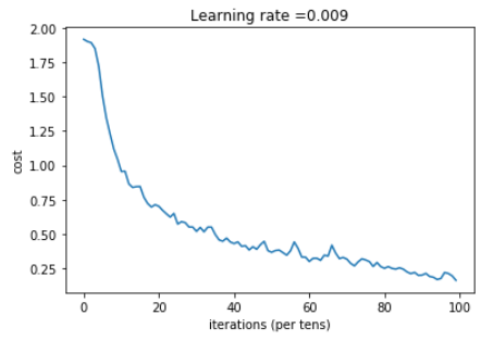
Tensor("Mean_1:0", shape=(), dtype=float32)
Train Accuracy: 0.940741
Test Accuracy: 0.783333

Expected output: although it may not match perfectly, your expected output should be close to ours and your cost value should decrease.

Cost after epoch 0 =    1.917929
Cost after epoch 5 =    1.506757
Train Accuracy =    0.940741
Test Accuracy =    0.783333

Congratulations! You have finised the assignment and built a model that recognizes SIGN language with almost 80% accuracy on the test set. If you wish, feel free to play around with this dataset further. You can actually improve its accuracy by spending more time tuning the hyperparameters, or using regularization (as this model clearly has a high variance).

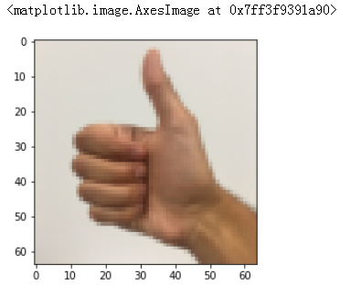
Once again, here's a thumbs up for your work! （再次, 为您的工作竖起大拇指!)

【code】

fname = "images/thumbs_up.jpg"
image = np.array(ndimage.imread(fname, flatten=False))
my_image = scipy.misc.imresize(image, size=(64,64))
plt.imshow(my_image)

【result】