Regression：Generalized Linear Models

作者：桂。

时间：2017-05-22  15:28:43

链接：http://www.cnblogs.com/xingshansi/p/6890048.html

---

前言

主要记录python工具包：sci-kit learn的基本用法。

本文主要是线性回归模型，包括：

　　1）普通最小二乘拟合

　　2）Ridge回归

　　3）Lasso回归

　　4）其他常用Linear Models.

一、普通最小二乘

通常是给定数据X,y，利用参数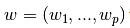进行线性拟合，准则为最小误差：

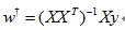
该问题的求解可以借助：梯度下降法/最小二乘法，以最小二乘为例：

基本用法：

from sklearn import linear_model
reg = linear_model.LinearRegression()
reg.fit ([[0, 0], [1, 1], [2, 2]], [0, 1, 2]) #拟合
reg.coef_#拟合结果
reg.predict(testdata) #预测

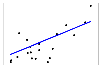
给出一个利用training data训练模型，并对test data预测的例子：

# -*- coding: utf-8 -*-
"""
Created on Mon May 22 15:26:03 2017

@author: Nobleding
"""

print(__doc__)

# Code source: Jaques Grobler
# License: BSD 3 clause

import matplotlib.pyplot as plt
import numpy as np
from sklearn import datasets, linear_model
from sklearn.metrics import mean_squared_error, r2_score

# Load the diabetes dataset
diabetes = datasets.load_diabetes()

# Use only one feature
diabetes_X = diabetes.data[:, np.newaxis, 2]

# Split the data into training/testing sets
diabetes_X_train = diabetes_X[:-20]
diabetes_X_test = diabetes_X[-20:]

# Split the targets into training/testing sets
diabetes_y_train = diabetes.target[:-20]
diabetes_y_test = diabetes.target[-20:]

# Create linear regression object
regr = linear_model.LinearRegression()

# Train the model using the training sets
regr.fit(diabetes_X_train, diabetes_y_train)

# Make predictions using the testing set
diabetes_y_pred = regr.predict(diabetes_X_test)

# The coefficients
print('Coefficients: \n', regr.coef_)
# The mean squared error
print("Mean squared error: %.2f"
      % mean_squared_error(diabetes_y_test, diabetes_y_pred))
# Explained variance score: 1 is perfect prediction
print('Variance score: %.2f' % r2_score(diabetes_y_test, diabetes_y_pred))

# Plot outputs
plt.scatter(diabetes_X_test, diabetes_y_test,  color='black')
plt.plot(diabetes_X_test, diabetes_y_pred, color='blue', linewidth=3)

plt.xticks(())
plt.yticks(())

plt.show()

二、Ridge回归

Ridge是在普通最小二乘的基础上添加正则项：

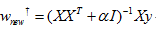
同样可以利用最小二乘求解：

基本用法：

from sklearn import linear_model
reg = linear_model.Ridge (alpha = .5)
reg.fit ([[0, 0], [0, 0], [1, 1]], [0, .1, 1])

　 给出一个W随α变化的例子：

print(__doc__)

import numpy as np
import matplotlib.pyplot as plt
from sklearn import linear_model

# X is the 10x10 Hilbert matrix
X = 1. / (np.arange(1, 11) + np.arange(0, 10)[:, np.newaxis])
y = np.ones(10)
n_alphas = 200
alphas = np.logspace(-10, -2, n_alphas)

coefs = []
for a in alphas:
    ridge = linear_model.Ridge(alpha=a, fit_intercept=False)
    ridge.fit(X, y)
    coefs.append(ridge.coef_)

ax = plt.gca()

ax.plot(alphas, coefs)
ax.set_xscale('log')
ax.set_xlim(ax.get_xlim()[::-1])  # reverse axis
plt.xlabel('alpha')
plt.ylabel('weights')
plt.title('Ridge coefficients as a function of the regularization')
plt.axis('tight')
plt.show()

　　可以看出alpha越小，w越大：

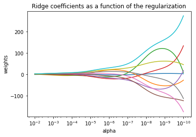
由于存在约束，何时最优呢？一个有效的方式是利用较差验证进行选取，利用Generalized Cross-Validation (GCV)：

from sklearn import linear_model
reg = linear_model.RidgeCV(alphas=[0.1, 1.0, 10.0])
reg.fit([[0, 0], [0, 0], [1, 1]], [0, .1, 1])
reg.alpha_

　

三、Lasso回归

其实添加约束项可以推而广之：

p = 2就是Ridge回归，p = 1就是Lasso回归。

给出Lasso的准则函数：

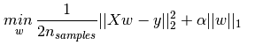
基本用法：

from sklearn import linear_model
reg = linear_model.Lasso(alpha = 0.1)
reg.fit([[0, 0], [1, 1]], [0, 1])
reg.predict([[1, 1]])

　

四、ElasticNet

其实就是Lasso与Ridge的折中：

基本用法：

from sklearn.linear_model import ElasticNet
enet = ElasticNet(alpha=alpha, l1_ratio=0.7)
y_pred_enet = enet.fit(X_train, y_train).predict(X_test)

　给出信号有Lasso以及ElasticNet回归的对比：

"""
========================================
Lasso and Elastic Net for Sparse Signals
========================================

Estimates Lasso and Elastic-Net regression models on a manually generated
sparse signal corrupted with an additive noise. Estimated coefficients are
compared with the ground-truth.

"""
print(__doc__)

import numpy as np
import matplotlib.pyplot as plt

from sklearn.metrics import r2_score

###############################################################################
# generate some sparse data to play with
np.random.seed(42)

n_samples, n_features = 50, 200
X = np.random.randn(n_samples, n_features)
coef = 3 * np.random.randn(n_features)
inds = np.arange(n_features)
np.random.shuffle(inds)
coef[inds[10:]] = 0  # sparsify coef
y = np.dot(X, coef)

# add noise
y += 0.01 * np.random.normal(size=n_samples)

# Split data in train set and test set
n_samples = X.shape[0]
X_train, y_train = X[:n_samples // 2], y[:n_samples // 2]
X_test, y_test = X[n_samples // 2:], y[n_samples // 2:]

###############################################################################
# Lasso
from sklearn.linear_model import Lasso

alpha = 0.1
lasso = Lasso(alpha=alpha)

y_pred_lasso = lasso.fit(X_train, y_train).predict(X_test)
r2_score_lasso = r2_score(y_test, y_pred_lasso)
print(lasso)
print("r^2 on test data : %f" % r2_score_lasso)

###############################################################################
# ElasticNet
from sklearn.linear_model import ElasticNet

enet = ElasticNet(alpha=alpha, l1_ratio=0.7)

y_pred_enet = enet.fit(X_train, y_train).predict(X_test)
r2_score_enet = r2_score(y_test, y_pred_enet)
print(enet)
print("r^2 on test data : %f" % r2_score_enet)

plt.plot(enet.coef_, color='lightgreen', linewidth=2,
         label='Elastic net coefficients')
plt.plot(lasso.coef_, color='gold', linewidth=2,
         label='Lasso coefficients')
plt.plot(coef, '--', color='navy', label='original coefficients')
plt.legend(loc='best')
plt.title("Lasso R^2: %f, Elastic Net R^2: %f"
          % (r2_score_lasso, r2_score_enet))
plt.show()

　　Lasso比Elastic是要稀疏一些的：

　

五、Lasso回归求解

实际应用中，Lasso求解是一类问题——稀疏重构（Sparse reconstrction），顺便总结一下。

对于欠定方程：其中，且，此时存在无穷多解，希望求解最稀疏的解：

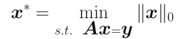
大牛们已经证明：当矩阵A满足限制等距属性（Restricted isometry propety, RIP）条件时，上述问题可松弛为：

RIP条件（更多细节点击这里）：

若y存在加性白噪声：，则上述问题可以有三种处理形式（某种程度等效，未研究）：

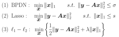
就是这几个问题都可以互相转化求解，以Lasso为例：这类方法很多，如投影梯度算法（Gradient Projection）、最小角回归（LARS）算法。

六、几种回归的联系

事实上，对于线性回归模型：

y = Wx + ε

ε为估计误差。

　　A-W为均匀分布（最小均方误差）

也就是：

　　B-W服从高斯分布（Ridge回归）

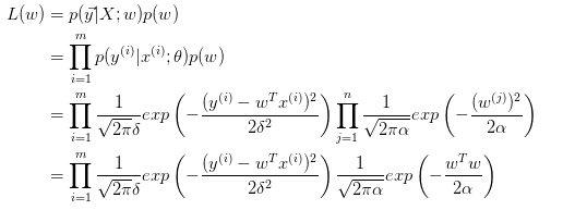
取对数：

等价于：

　　C-W服从拉普拉斯分布（Lasso回归）

与Ridge推导类似，得出：

三种情况对应的约束边界：

最小二乘：均匀分布就是无约束的情况。

Ridge：

Lasso:

这样对应图形来看就更明显了，可以看出对W的约束是越来越严格的。ElasticNet的情况虽然没有分析，也容易理解：它的限定条件一定介于菱形与圆形两边界之间。

七、其他

更多的拟合可以看链接，用到了补充了，这里列几个以前见过的。

　　A-最小角回归（Least Angle Regressive，LARS）

LARS算法点击这里。

基本用法：

from sklearn import linear_model
clf = linear_model.Lars(n_nonzero_coefs=1)
clf.fit([[-1, 1], [0, 0], [1, 1]], [-1.1111, 0, -1.1111])
print(clf.coef_) 

　　B-正交匹配追踪（orthogonal matching pursuit, OMP）

OMP思路：

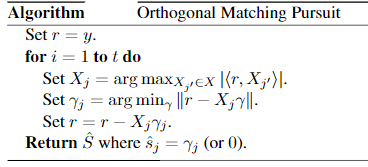
对应准则函数：

也可以写为：

本质上是对重建信号，不断从字典中找出最匹配的基，然后进行表达，表达后的残差：再从字典中找基进行表达，循环往复。

停止的基本条件通常有三类：1）达到指定的迭代次数;2）残差小于给定的门限;3）字典的任意基与残差的相关性小于给定的门限.

基本用法：

"""
===========================
Orthogonal Matching Pursuit
===========================

Using orthogonal matching pursuit for recovering a sparse signal from a noisy
measurement encoded with a dictionary
"""
print(__doc__)

import matplotlib.pyplot as plt
import numpy as np
from sklearn.linear_model import OrthogonalMatchingPursuit
from sklearn.linear_model import OrthogonalMatchingPursuitCV
from sklearn.datasets import make_sparse_coded_signal

n_components, n_features = 512, 100
n_nonzero_coefs = 17

# generate the data
###################

# y = Xw
# |x|_0 = n_nonzero_coefs

y, X, w = make_sparse_coded_signal(n_samples=1,
                                   n_components=n_components,
                                   n_features=n_features,
                                   n_nonzero_coefs=n_nonzero_coefs,
                                   random_state=0)

idx, = w.nonzero()

# distort the clean signal
##########################
y_noisy = y + 0.05 * np.random.randn(len(y))

# plot the sparse signal
########################
plt.figure(figsize=(7, 7))
plt.subplot(4, 1, 1)
plt.xlim(0, 512)
plt.title("Sparse signal")
plt.stem(idx, w[idx])

# plot the noise-free reconstruction
####################################

omp = OrthogonalMatchingPursuit(n_nonzero_coefs=n_nonzero_coefs)
omp.fit(X, y)
coef = omp.coef_
idx_r, = coef.nonzero()
plt.subplot(4, 1, 2)
plt.xlim(0, 512)
plt.title("Recovered signal from noise-free measurements")
plt.stem(idx_r, coef[idx_r])

# plot the noisy reconstruction
###############################
omp.fit(X, y_noisy)
coef = omp.coef_
idx_r, = coef.nonzero()
plt.subplot(4, 1, 3)
plt.xlim(0, 512)
plt.title("Recovered signal from noisy measurements")
plt.stem(idx_r, coef[idx_r])

# plot the noisy reconstruction with number of non-zeros set by CV
##################################################################
omp_cv = OrthogonalMatchingPursuitCV()
omp_cv.fit(X, y_noisy)
coef = omp_cv.coef_
idx_r, = coef.nonzero()
plt.subplot(4, 1, 4)
plt.xlim(0, 512)
plt.title("Recovered signal from noisy measurements with CV")
plt.stem(idx_r, coef[idx_r])

plt.subplots_adjust(0.06, 0.04, 0.94, 0.90, 0.20, 0.38)
plt.suptitle('Sparse signal recovery with Orthogonal Matching Pursuit',
             fontsize=16)
plt.show()

　　结果图：

　　C-贝叶斯回归（Bayesian Regression）

其实就是将最小二乘的拟合问题转化为概率问题：

上面分析几种回归关系的时候，概率的部分就是贝叶斯回归的思想。

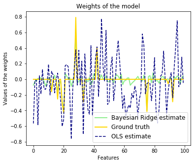
为什么贝叶斯回归可以避免overfitting？MLE对应最小二乘拟合，Bayessian Regression对应有约束的拟合，这个约束也就是先验概率。

基本用法：

clf = BayesianRidge(compute_score=True)
clf.fit(X, y)

　　代码示例：

"""
=========================
Bayesian Ridge Regression
=========================

Computes a Bayesian Ridge Regression on a synthetic dataset.

See :ref:`bayesian_ridge_regression` for more information on the regressor.

Compared to the OLS (ordinary least squares) estimator, the coefficient
weights are slightly shifted toward zeros, which stabilises them.

As the prior on the weights is a Gaussian prior, the histogram of the
estimated weights is Gaussian.

The estimation of the model is done by iteratively maximizing the
marginal log-likelihood of the observations.

We also plot predictions and uncertainties for Bayesian Ridge Regression
for one dimensional regression using polynomial feature expansion.
Note the uncertainty starts going up on the right side of the plot.
This is because these test samples are outside of the range of the training
samples.
"""
print(__doc__)

import numpy as np
import matplotlib.pyplot as plt
from scipy import stats

from sklearn.linear_model import BayesianRidge, LinearRegression

###############################################################################
# Generating simulated data with Gaussian weights
np.random.seed(0)
n_samples, n_features = 100, 100
X = np.random.randn(n_samples, n_features)  # Create Gaussian data
# Create weights with a precision lambda_ of 4.
lambda_ = 4.
w = np.zeros(n_features)
# Only keep 10 weights of interest
relevant_features = np.random.randint(0, n_features, 10)
for i in relevant_features:
    w[i] = stats.norm.rvs(loc=0, scale=1. / np.sqrt(lambda_))
# Create noise with a precision alpha of 50.
alpha_ = 50.
noise = stats.norm.rvs(loc=0, scale=1. / np.sqrt(alpha_), size=n_samples)
# Create the target
y = np.dot(X, w) + noise

###############################################################################
# Fit the Bayesian Ridge Regression and an OLS for comparison
clf = BayesianRidge(compute_score=True)
clf.fit(X, y)

ols = LinearRegression()
ols.fit(X, y)

###############################################################################
# Plot true weights, estimated weights, histogram of the weights, and
# predictions with standard deviations
lw = 2
plt.figure(figsize=(6, 5))
plt.title("Weights of the model")
plt.plot(clf.coef_, color='lightgreen', linewidth=lw,
         label="Bayesian Ridge estimate")
plt.plot(w, color='gold', linewidth=lw, label="Ground truth")
plt.plot(ols.coef_, color='navy', linestyle='--', label="OLS estimate")
plt.xlabel("Features")
plt.ylabel("Values of the weights")
plt.legend(loc="best", prop=dict(size=12))

　　D-多项式回归（Polynomial regression）

上文的最小二乘拟合可以理解成多元回归问题。多项式回归可以转化为多元回归问题。

对于

令

则

这就是多元回归问题了。

基本用法（阶数需指定）：

print(__doc__)

# Author: Mathieu Blondel
#         Jake Vanderplas
# License: BSD 3 clause

import numpy as np
import matplotlib.pyplot as plt

from sklearn.linear_model import Ridge
from sklearn.preprocessing import PolynomialFeatures
from sklearn.pipeline import make_pipeline

def f(x):
    """ function to approximate by polynomial interpolation"""
    return x * np.sin(x)

# generate points used to plot
x_plot = np.linspace(0, 10, 100)

# generate points and keep a subset of them
x = np.linspace(0, 10, 100)
rng = np.random.RandomState(0)
rng.shuffle(x)
x = np.sort(x[:20])
y = f(x)

# create matrix versions of these arrays
X = x[:, np.newaxis]
X_plot = x_plot[:, np.newaxis]

colors = ['teal', 'yellowgreen', 'gold']
lw = 2
plt.plot(x_plot, f(x_plot), color='cornflowerblue', linewidth=lw,
         label="ground truth")
plt.scatter(x, y, color='navy', s=30, marker='o', label="training points")

for count, degree in enumerate([3, 4, 5]):
    model = make_pipeline(PolynomialFeatures(degree), Ridge())
    model.fit(X, y)
    y_plot = model.predict(X_plot)
    plt.plot(x_plot, y_plot, color=colors[count], linewidth=lw,
             label="degree %d" % degree)

plt.legend(loc='lower left')

plt.show()

　　E-罗杰斯特回归（Logistic regression）

这个之前有梳理过。

L2约束（就是softmax衰减的情况）：

也可以是L1约束：

基本用法：

"""
==============================================
L1 Penalty and Sparsity in Logistic Regression
==============================================

Comparison of the sparsity (percentage of zero coefficients) of solutions when
L1 and L2 penalty are used for different values of C. We can see that large
values of C give more freedom to the model.  Conversely, smaller values of C
constrain the model more. In the L1 penalty case, this leads to sparser
solutions.

We classify 8x8 images of digits into two classes: 0-4 against 5-9.
The visualization shows coefficients of the models for varying C.
"""

print(__doc__)

# Authors: Alexandre Gramfort <alexandre.gramfort@inria.fr>
#          Mathieu Blondel <mathieu@mblondel.org>
#          Andreas Mueller <amueller@ais.uni-bonn.de>
# License: BSD 3 clause

import numpy as np
import matplotlib.pyplot as plt

from sklearn.linear_model import LogisticRegression
from sklearn import datasets
from sklearn.preprocessing import StandardScaler

digits = datasets.load_digits()

X, y = digits.data, digits.target
X = StandardScaler().fit_transform(X)

# classify small against large digits
y = (y > 4).astype(np.int)

# Set regularization parameter
for i, C in enumerate((100, 1, 0.01)):
    # turn down tolerance for short training time
    clf_l1_LR = LogisticRegression(C=C, penalty='l1', tol=0.01)
    clf_l2_LR = LogisticRegression(C=C, penalty='l2', tol=0.01)
    clf_l1_LR.fit(X, y)
    clf_l2_LR.fit(X, y)

    coef_l1_LR = clf_l1_LR.coef_.ravel()
    coef_l2_LR = clf_l2_LR.coef_.ravel()

    # coef_l1_LR contains zeros due to the
    # L1 sparsity inducing norm

    sparsity_l1_LR = np.mean(coef_l1_LR == 0) * 100
    sparsity_l2_LR = np.mean(coef_l2_LR == 0) * 100

    print("C=%.2f" % C)
    print("Sparsity with L1 penalty: %.2f%%" % sparsity_l1_LR)
    print("score with L1 penalty: %.4f" % clf_l1_LR.score(X, y))
    print("Sparsity with L2 penalty: %.2f%%" % sparsity_l2_LR)
    print("score with L2 penalty: %.4f" % clf_l2_LR.score(X, y))

    l1_plot = plt.subplot(3, 2, 2 * i + 1)
    l2_plot = plt.subplot(3, 2, 2 * (i + 1))
    if i == 0:
        l1_plot.set_title("L1 penalty")
        l2_plot.set_title("L2 penalty")

    l1_plot.imshow(np.abs(coef_l1_LR.reshape(8, 8)), interpolation='nearest',
                   cmap='binary', vmax=1, vmin=0)
    l2_plot.imshow(np.abs(coef_l2_LR.reshape(8, 8)), interpolation='nearest',
                   cmap='binary', vmax=1, vmin=0)
    plt.text(-8, 3, "C = %.2f" % C)

    l1_plot.set_xticks(())
    l1_plot.set_yticks(())
    l2_plot.set_xticks(())
    l2_plot.set_yticks(())

plt.show()

　　8X8的figure，不同C取值：

　　F-随机梯度下降（Stochastic Gradient Descent, SGD）

梯度下降之前梳理过了。

基本用法：

from sklearn.linear_model import SGDClassifier
X = [[0., 0.], [1., 1.]]
y = [0, 1]
clf = SGDClassifier(loss="hinge", penalty="l2")
clf.fit(X, y)

　　其中涉及到：SGDClassifier，Linear classifiers (SVM, logistic regression, a.o.) with SGD training.提供了分类与回归的应用：

The classes SGDClassifier and SGDRegressor provide functionality to fit linear models for classification and regression using different (convex) loss functions and different penalties. E.g., with loss="log", SGDClassifier fits a logistic regression model, while with loss="hinge" it fits a linear support vector machine (SVM).

以分类为例：

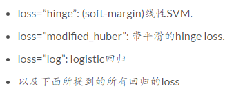
clf = SGDClassifier(loss="log").fit(X, y)

其中loss:

 'hinge', 'log', 'modified_huber', 'squared_hinge',\
                'perceptron', or a regression loss: 'squared_loss', 'huber',\
                'epsilon_insensitive', or 'squared_epsilon_insensitive'

　　应用实例：

print(__doc__)

import numpy as np
import matplotlib.pyplot as plt
from sklearn import datasets
from sklearn.linear_model import SGDClassifier

# import some data to play with
iris = datasets.load_iris()
X = iris.data[:, :2]  # we only take the first two features. We could
                      # avoid this ugly slicing by using a two-dim dataset
y = iris.target
colors = "bry"

# shuffle
idx = np.arange(X.shape[0])
np.random.seed(13)
np.random.shuffle(idx)
X = X[idx]
y = y[idx]

# standardize
mean = X.mean(axis=0)
std = X.std(axis=0)
X = (X - mean) / std

h = .02  # step size in the mesh

clf = SGDClassifier(alpha=0.001, n_iter=100).fit(X, y)

# create a mesh to plot in
x_min, x_max = X[:, 0].min() - 1, X[:, 0].max() + 1
y_min, y_max = X[:, 1].min() - 1, X[:, 1].max() + 1
xx, yy = np.meshgrid(np.arange(x_min, x_max, h),
                     np.arange(y_min, y_max, h))

# Plot the decision boundary. For that, we will assign a color to each
# point in the mesh [x_min, x_max]x[y_min, y_max].
Z = clf.predict(np.c_[xx.ravel(), yy.ravel()])
# Put the result into a color plot
Z = Z.reshape(xx.shape)
cs = plt.contourf(xx, yy, Z, cmap=plt.cm.Paired)
plt.axis('tight')

# Plot also the training points
for i, color in zip(clf.classes_, colors):
    idx = np.where(y == i)
    plt.scatter(X[idx, 0], X[idx, 1], c=color, label=iris.target_names[i],
                cmap=plt.cm.Paired)
plt.title("Decision surface of multi-class SGD")
plt.axis('tight')

# Plot the three one-against-all classifiers
xmin, xmax = plt.xlim()
ymin, ymax = plt.ylim()
coef = clf.coef_
intercept = clf.intercept_

def plot_hyperplane(c, color):
    def line(x0):
        return (-(x0 * coef[c, 0]) - intercept[c]) / coef[c, 1]

    plt.plot([xmin, xmax], [line(xmin), line(xmax)],
             ls="--", color=color)

for i, color in zip(clf.classes_, colors):
    plot_hyperplane(i, color)
plt.legend()
plt.show()

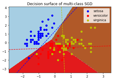
　　G-感知器（Perceptron）

之前梳理过。SGDClassifier中包含Perceptron。

　　H-随机采样一致（Random sample consensus, RANSAC）

之前梳理过。Ransac是数据预处理的操作。

基本用法：

ransac = linear_model.RANSACRegressor()
ransac.fit(X, y)

　　应用实例：

import numpy as np
from matplotlib import pyplot as plt

from sklearn import linear_model, datasets

n_samples = 1000
n_outliers = 50

X, y, coef = datasets.make_regression(n_samples=n_samples, n_features=1,
                                      n_informative=1, noise=10,
                                      coef=True, random_state=0)

# Add outlier data
np.random.seed(0)
X[:n_outliers] = 3 + 0.5 * np.random.normal(size=(n_outliers, 1))
y[:n_outliers] = -3 + 10 * np.random.normal(size=n_outliers)

# Fit line using all data
lr = linear_model.LinearRegression()
lr.fit(X, y)

# Robustly fit linear model with RANSAC algorithm
ransac = linear_model.RANSACRegressor()
ransac.fit(X, y)
inlier_mask = ransac.inlier_mask_
outlier_mask = np.logical_not(inlier_mask)

# Predict data of estimated models
line_X = np.arange(X.min(), X.max())[:, np.newaxis]
line_y = lr.predict(line_X)
line_y_ransac = ransac.predict(line_X)

# Compare estimated coefficients
print("Estimated coefficients (true, linear regression, RANSAC):")
print(coef, lr.coef_, ransac.estimator_.coef_)

lw = 2
plt.scatter(X[inlier_mask], y[inlier_mask], color='yellowgreen', marker='.',
            label='Inliers')
plt.scatter(X[outlier_mask], y[outlier_mask], color='gold', marker='.',
            label='Outliers')
plt.plot(line_X, line_y, color='navy', linewidth=lw, label='Linear regressor')
plt.plot(line_X, line_y_ransac, color='cornflowerblue', linewidth=lw,
         label='RANSAC regressor')
plt.legend(loc='lower right')
plt.xlabel("Input")
plt.ylabel("Response")
plt.show()

参考：

• http://scikit-learn.org/dev/supervised_learning.html#supervised-learning
• https://www.zhihu.com/question/23536142