[Scikit-learn] 1.5 Generalized Linear Models

梯度下降

一、亲手实现“梯度下降”

以下内容其实就是《手动实现简单的梯度下降》。

神经网络的实践笔记，主要包括：

Logistic分类函数

反向传播相关内容

Link: http://peterroelants.github.io/posts/neural_network_implementation_part01/

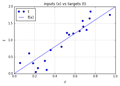
中文版: http://www.jianshu.com/p/0da9eb3fd06b

1. 生成训练数据

由“目标函数+随机噪声”生成。

import numpy as np

import matplotlib.pyplot as plt

# Part 1, create training data

# Define the vector of input samples as x, with 20 values sampled from a uniform distribution

# between 0 and 1
x = np.random.uniform(0, 1, 20)

# Generate the target values t from x with small gaussian noise so the estimation won't be perfect.

# Define a function f that represents the line that generates t without noise

def f(x): return x * 2

# Create the targets t with some gaussian noise

noise_variance = 0.2 # Variance of the gaussian noise

# Gaussian noise error for each sample in x
# shape函数是numpy.core.fromnumeric中的函数，它的功能是读取矩阵的长度，比如shape[0]就是读取矩阵第一维度的长度。
# shape[0]得到对应的长度，也即是真实值的个数，以便生成对应的noise值
noise = np.random.randn(x.shape[0]) * noise_variance

# Create targets t

t = f(x) + noise


# Part2, draw the training data

# Plot the target t versus the input x

plt.plot(x, t, 'o', label='t')

# Plot the initial line

plt.plot([0, 1], [f(0), f(1)], 'b-', label='f(x)')

plt.xlabel('$x$', fontsize=15)

plt.ylabel('$t$', fontsize=15)

plt.ylim([0,2])

plt.title('inputs (x) vs targets (t)')

plt.grid()

plt.legend(loc=2)

plt.show()

2. loss与weight的关系

# 定义“神经网络模型“

def nn(x, w): return x*w

# 定义“损失函数”

def cost(y, t): return ((t - y) ** 2).sum()

# Plot the cost vs the given weight w

# Define a vector of weights for which we want to plot the cost
# start 是采样的起始点
# stop  是采样的终点
# num   是采样的点个数
ws = np.linspace(0, 4, num=100)  # weight values

cost_ws = np.vectorize(lambda w: cost(nn(x, w) , t))(ws)  # cost for each weight in ws

# Plot

plt.plot(ws, cost_ws, 'r-')

plt.xlabel('$w$', fontsize=15)

plt.ylabel('$\\xi$', fontsize=15)

plt.title('cost vs. weight')

plt.grid()

plt.show()

3. 梯度模拟

# define the gradient function. Remember that y = nn(x, w) = x * w

def gradient(w, x, t):

    return 2 * x * (nn(x, w) - t)

# define the update function delta w

def delta_w(w_k, x, t, learning_rate):

    return learning_rate * gradient(w_k, x, t).sum()

# Set the initial weight parameter

w = 0.1

# Set the learning rate

learning_rate = 0.1

# Start performing the gradient descent updates, and print the weights and cost:

nb_of_iterations = 4  # number of gradient descent updates

w_cost = [(w, cost(nn(x, w), t))] # List to store the weight,costs values

for i in range(nb_of_iterations):

    dw = delta_w(w, x, t, learning_rate)   # Get the delta w update

    w  = w - dw                            # Update the current weight parameter

    w_cost.append((w, cost(nn(x, w), t)))  # Add weight,cost to list

# Print the final w, and cost

for i in range(0, len(w_cost)):

    print('w({}): {:.4f} \t cost: {:.4f}'.format(i, w_cost[i][0], w_cost[i][1]))



# Plot the first 2 gradient descent updates

plt.plot(ws, cost_ws, 'r-')  # Plot the error curve

# Plot the updates

for i in range(0, len(w_cost)-2):

    w1, c1 = w_cost[i]

    w2, c2 = w_cost[i+1]

    plt.plot(w1, c1, 'bo')

    plt.plot([w1, w2],[c1, c2], 'b-')

    plt.text(w1, c1+0.5, '$w({})$'.format(i))

# Show figure

plt.xlabel('$w$', fontsize=15)

plt.ylabel('$\\xi$', fontsize=15)

plt.title('Gradient descent updates plotted on cost function')

plt.grid()

plt.show()

w(0): 0.1000 cost: 25.1338
w(1): 2.5774 cost: 2.7926
w(2): 1.9036 cost: 1.1399
w(3): 2.0869 cost: 1.0177
w(4): 2.0370 cost: 1.0086

4. 预测的效果

w = 0

# Start performing the gradient descent updates

nb_of_iterations = 10  # number of gradient descent updates

for i in range(nb_of_iterations):

    dw = delta_w(w, x, t, learning_rate)  # get the delta w update

    w = w - dw  # update the current weight parameter

# Plot the fitted line agains the target line

# Plot the target t versus the input x

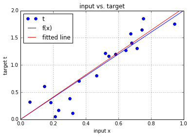
plt.plot(x, t, 'o', label='t')

# Plot the initial line

plt.plot([0, 1], [f(0), f(1)], 'b-', label='f(x)')

# plot the fitted line

plt.plot([0, 1], [0*w, 1*w], 'r-', label='fitted line')

plt.xlabel('input x')

plt.ylabel('target t')

plt.ylim([0,2])

plt.title('input vs. target')

plt.grid()

plt.legend(loc=2)

plt.show()

二、封装在API

以上是实现细节，在scikit-learn中被封装成了如下精简的API。

Ref: [Scikit-learn] 1.1. Generalized Linear Models - Neural network models

mlp = MLPClassifier(verbose=0, random_state=0, max_iter=max_iter, **param)

mlp.fit(X, y)

mlps.append(mlp)

随机梯度下降

一、基本介绍

Ref: 1.5. Stochastic Gradient Descent

Stochastic Gradient Descent (SGD) is a simple yet very efficient approach to discriminative learning of linear classifiers under convex loss functions such as (linear) Support Vector Machines and Logistic Regression.

- Logistic Regression 是模型
- SGD 是算法，也就是 “The solver for weight optimization.” 权重优化方法。

SGD has been successfully applied to large-scale and sparse machine learning problems often encountered in text classification and natural language processing.

Given that the data is sparse, the classifiers in this module easily scale to problems with more than 10^5 training examples and more than 10^5 features.

nlp Feature:

- Loss function: 凸
- 数据大且稀疏（维度高）

The advantages of Stochastic Gradient Descent are:

Efficiency.

Ease of implementation (lots of opportunities for code tuning).

The disadvantages of Stochastic Gradient Descent include:

SGD requires a number of hyperparameters such as the regularization parameter and the number of iterations.

SGD is sensitive to feature scaling.

二、函数接口

1.5. Stochastic Gradient Descent

函数名

SGDRegressor 类实现了一个简单的随机梯度下降的学习算法的程序，该程序支持不同的损失函数和罚项来拟合线性回归模型。

- SGDRegressor 对于非常大的训练样本(>10.000)的回归问题是非常合适的。
- 对于其他问题我们推荐 Ridge, Lasso 或者 ElasticNet 。

函数参数

具体损失函数可以通过设置 loss 参数。 SGDRegressor 支持以下几种损失函数:

- loss="squared_loss": Ordinary least squares,　　// 可以用于鲁棒回归
- loss="huber": Huber loss for robust regression,　　// 可以用于鲁棒回归
- loss="epsilon_insensitive": linear Support Vector Regression.　　// insensitive区域的宽度可以通过参数 epsilon 指定，该参数由目标变量的规模来决定。

三、模型比较

SGDRegressor 和 SGDClassifier 一样支持平均SGD。Averaging 可以通过设置 `average=True` 来启用。

对于带平方损失和L2罚项的回归，提供了另外一个带平均策略的SGD的变体，使用了随机平均梯度算法(SAG), 实现程序为Ridge 。 # 难道不是直接套公式？而是采用逼近法估参？

问题来了：from sklearn.linear_model import LinearRegression, Lasso, Ridge, ElasticNet, SGDRegressor

前四种方法：LinearRegression, Lasso, Ridge, ElasticNet

from sklearn.cross_validation import KFold

from sklearn.linear_model import LinearRegression, Lasso, Ridge, ElasticNet, SGDRegressor

import numpy as np

from sklearn.datasets import load_boston

boston = load_boston()

np.set_printoptions(precision=2, linewidth=120, suppress=True, edgeitems=4)

# In order to do multiple regression we need to add a column of 1s for x0

x = np.array([np.concatenate((v,[1])) for v in boston.data])

y = boston.target

a = 0.3

for name,met in [

        ('linear regression', LinearRegression()),

        ('lasso', Lasso(fit_intercept=True, alpha=a)),

        ('ridge', Ridge(fit_intercept=True, alpha=a)),

        ('elastic-net', ElasticNet(fit_intercept=True, alpha=a))

        ]:

    met.fit(x,y)

    # p = np.array([met.predict(xi) for xi in x])

    p = met.predict(x)

    e = p-y

    total_error = np.dot(e,e)

    rmse_train = np.sqrt(total_error/len(p))

    kf = KFold(len(x), n_folds=10)

    err = 0

    for train,test in kf:

        met.fit(x[train],y[train])

        p = met.predict(x[test])

        e = p-y[test]

        err += np.dot(e,e)

    rmse_10cv = np.sqrt(err/len(x))

    print('Method: %s' %name)

    print('RMSE on training: %.4f' %rmse_train)

    print('RMSE on 10-fold CV: %.4f' %rmse_10cv)

    print("\n")

Method: linear regression

RMSE on training: 4.6795

RMSE on 10-fold CV: 5.8819

Method: lasso

RMSE on training: 4.8570

RMSE on 10-fold CV: 5.7675

Method: ridge

RMSE on training: 4.6822

RMSE on 10-fold CV: 5.8535

Method: elastic-net

RMSE on training: 4.9072

RMSE on 10-fold CV: 5.4936

Stochastic Gradient Descent 实践

# SGD is very senstitive to varying-sized feature values. So, first we need to do feature scaling.

from sklearn.preprocessing import StandardScaler

scaler = StandardScaler()

scaler.fit(x)

x_s == SGDRegressor(penalty='l2', alpha=0.15, n_iter=200)

sgdreg.fit(x_s,y)

p = sgdreg.predict(x_s)

err = p-y

total_error = np.dot(err,err)

rmse_train  = np.sqrt(total_error/len(p))

# Compute RMSE using 10-fold x-validation

kf = KFold(len(x), n_folds=10)

xval_err = 0

for train,test in kf:

    scaler   = StandardScaler()

    scaler.fit(x[train])                  # Don't cheat - fit only on training data

    xtrain_s = scaler.transform(x[train])

    xtest_s  = scaler.transform(x[test])  # apply same transformation to test data

    sgdreg.fit(xtrain_s,y[train])

    p = sgdreg.predict(xtest_s)

    e = p-y[test]

    xval_err += np.dot(e,e)

rmse_10cv = np.sqrt(xval_err/len(x))

method_name = 'Stochastic Gradient Descent Regression'

print('Method: %s' %method_name)

print('RMSE on training: %.4f' %rmse_train)

print('RMSE on 10-fold CV: %.4f' %rmse_10cv)

Method: Stochastic Gradient Descent Regression

RMSE on training: 4.8119

RMSE on 10-fold CV: 5.5741

End.