矩池云 | 神经网络图像分割：气胸X光片识别案例

在上一次肺炎X光片的预测中,我们通过神经网络来识别患者胸部的X光片，用于检测患者是否患有肺炎。这是一个典型的神经网络图像分类在医学领域中的运用。

另外，神经网络的图像分割在医学领域中也有着很重要的用作。接下来，我们要演示如何在气胸患者的X光片上，分割出气胸患者患病区的部位和形状。

那么就让我们来正式开始了。

第一步：导入需要的 Python 包

import sys
import cv2
import pydicom

import numpy as np
import pandas as pd

import matplotlib.pyplot as plt
from matplotlib import patches as patches

from glob import glob
from tqdm import tqdm

from plotly.offline import download_plotlyjs, init_notebook_mode, iplot
from plotly import subplots
from plotly.graph_objs import *
from plotly.graph_objs.layout import Margin, YAxis, XAxis
init_notebook_mode()

import tensorflow as tf
from tensorflow import reduce_sum
from tensorflow.keras.models import Model
from tensorflow.keras.layers import Input, Conv2D, MaxPool2D, UpSampling2D, Concatenate, Flatten, Add
from tensorflow.keras.losses import binary_crossentropy
from tensorflow.keras import callbacks

from sklearn.model_selection import train_test_split

# 数据增强库
from albumentations import (
    Compose, HorizontalFlip, CLAHE, HueSaturationValue,
    RandomBrightness, RandomContrast, RandomGamma,OneOf,
    ToFloat, ShiftScaleRotate,GridDistortion, ElasticTransform, JpegCompression, HueSaturationValue,
    RGBShift, RandomBrightness, RandomContrast, Blur, MotionBlur, MedianBlur, GaussNoise,CenterCrop,
    IAAAdditiveGaussianNoise,GaussNoise,OpticalDistortion,RandomSizedCrop
)

# 设置使用90%的显存，避免显存OOM错误
config = tf.compat.v1.ConfigProto()
config.gpu_options.per_process_gpu_memory_fraction = 0.9
session = tf.compat.v1.Session(config=config)

%matplotlib inline

第二步：导入数据库

图像分割的数据一共分为两部分：

训练用的图片

图片中需要分割的部分，称之为 mask

这次我们训练的数据是以 DCM 文件存储。

DCM 是一种数位成像，广泛运用于医学领域，但并不局限于医学，DCM 本身是一种特殊的图像文件，它可以用来存储各种图像信息。

DCM 文件是遵循 DICOM 标准的一种文件

我们的 mask 部分的数据存储在 csv 文件中，csv 文件大家都比较熟悉, 这里就不做介绍了。

2.1 导入 mask 数据

首先我们来看下存放 mask 数据的 csv 文件中的 mask 数据

使用 pandas 的 read_csv 接口读取 train-rle.csv 文件。

我们先查看其中的头部5条数据，其中我们可以看到这个 csv 文件中存放了两列，一列是 ImageId ， 一列是 EncodedPixels 。

ImageId 这一列比较好理解，是训练数据的 id，对应的是 dcm 文件的文件名。

rles_df = pd.read_csv('pneumothorax-segmentation/train-rle.csv')
rles_df.columns = ['ImageId', 'EncodedPixels']
rles_df.head()

这里要对 EncodedPixels 这一列做下说明：

EncodedPixels 实际存放的就是 mask 的像素数据，这些像素数据是以 RLE 编码存放的。

接下来，我们需要定义一个函数来将 RLE 编码的数据还原成 mask 图片数据。

def rle2mask(rle, width, height):
    mask= np.zeros(width* height)
    array = np.asarray([int(x) for x in rle.split()])
    starts = array[0::2]
    lengths = array[1::2]

    current_position = 0
    for index, start in enumerate(starts):
        current_position += start
        mask[current_position:current_position+lengths[index]] = 255
        current_position += lengths[index]

    return mask.reshape(width, height)

2.2 导入 DCM 文件

接下来我们将DCM读入并存储到字典中，方便以后查看跟使用。我们还将之前读入的 mask 数据也合并到相应的 ImageId 的字典中。

在训练数据中，如果胸片没有被 mask 标记，表示这个病例他并不患有气胸。通过 EncodedPixels 中的数据，将是否是气胸的患者记录到 has_pneumothorax 这一字段中。

def dicom_to_dict(dicom_data, file_path, rles_df, encoded_pixels=True):
    data = {}

    # Parse fields with meaningful information
    data['patient_name'] = dicom_data.PatientName
    data['patient_id'] = dicom_data.PatientID
    data['patient_age'] = int(dicom_data.PatientAge)
    data['patient_sex'] = dicom_data.PatientSex
    data['pixel_spacing'] = dicom_data.PixelSpacing
    data['file_path'] = file_path
    data['id'] = dicom_data.SOPInstanceUID

    # look for annotation if enabled (train set)
    if encoded_pixels:
        encoded_pixels_list = rles_df[rles_df['ImageId']==dicom_data.SOPInstanceUID]['EncodedPixels'].values

        pneumothorax = False
        for encoded_pixels in encoded_pixels_list:
            if encoded_pixels != ' -1':
                pneumothorax = True

        data['encoded_pixels_list'] = encoded_pixels_list
        data['has_pneumothorax'] = pneumothorax
        data['encoded_pixels_count'] = len(encoded_pixels_list)

    return data

    train_fns = sorted(glob('pneumothorax-segmentation/dicom-images-train/*/*/*.dcm'))
train_metadata_df = pd.DataFrame()
train_metadata_list = []
for file_path in tqdm(train_fns):
    dicom_data = pydicom.dcmread(file_path)
    train_metadata = dicom_to_dict(dicom_data, file_path, rles_df)
    train_metadata_list.append(train_metadata)
train_metadata_df = pd.DataFrame(train_metadata_list)
train_metadata_df.head()

第三步：数据可视化

我们在读取完数据以后，接下来就进行数据情况的查看。

3.1 随机挑选病例样本

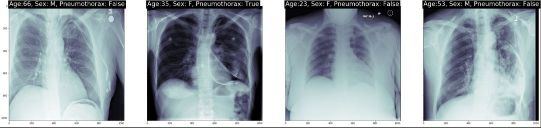
我们随机挑选了几个病例。我们在每个病例上打出了年龄，性别以及是否是气胸患者。

num_img = 4
subplot_count = 0
fig, ax = plt.subplots(nrows=1, ncols=num_img, sharey=True, figsize=(num_img*10,10))
for index, row in train_metadata_df.sample(n=num_img).iterrows():
    dataset = pydicom.dcmread(row['file_path'])
    ax[subplot_count].imshow(dataset.pixel_array, cmap=plt.cm.bone)
    # label the x-ray with information about the patient
    ax[subplot_count].text(0,0,'Age:{}, Sex: {}, Pneumothorax: {}'.format(row['patient_age'],row['patient_sex'],row['has_pneumothorax']),
                           size=26,color='white', backgroundcolor='black')
    subplot_count += 1

结果如图示：

我们在看下 mask 图像在相对应的病例中的位置：

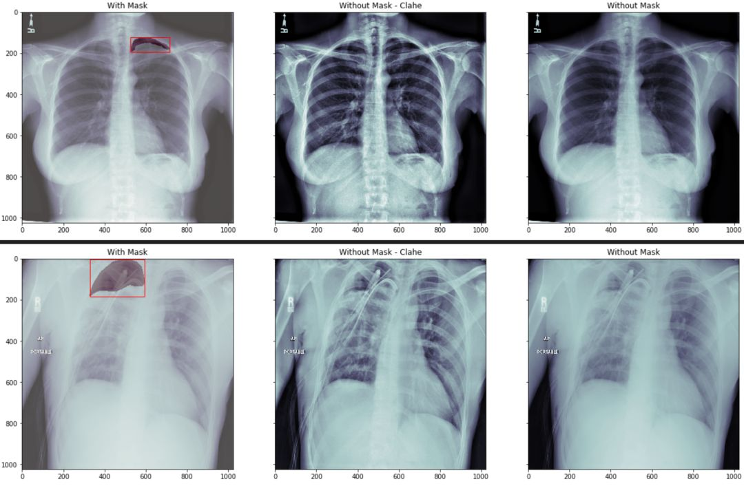
我们分三组来显示

第一组我们将原始胸片图像中用红色的框框出 mask 的最小包围盒. 然后将mask 数据部分用不同的颜色区分

第二组我们将原始图像做直方图均衡化处理，让胸片对比度更加清晰。

第三组我们直接显示原始图像

通过观察我们看到，如果没有一定的专业知识，根本无法区分跟看出气胸的具体位置。

def bounding_box(img):
    # return max and min of a mask to draw bounding box
    rows = np.any(img, axis=1)
    cols = np.any(img, axis=0)
    rmin, rmax = np.where(rows)[0][[0, -1]]
    cmin, cmax = np.where(cols)[0][[0, -1]]

    return rmin, rmax, cmin, cmax

def plot_with_mask_and_bbox(file_path, mask_encoded_list, figsize=(20,10)):
    pixel_array = pydicom.dcmread(file_path).pixel_array

    clahe = cv2.createCLAHE(clipLimit=2.0, tileGridSize=(16, 16))
    clahe_pixel_array = clahe.apply(pixel_array)

    # use the masking function to decode RLE
    mask_decoded_list = [rle2mask(mask_encoded, 1024, 1024).T for mask_encoded in mask_encoded_list]

    fig, ax = plt.subplots(nrows=1, ncols=3, sharey=True, figsize=(20,10))

    # print out the xray
    ax[0].imshow(pixel_array, cmap=plt.cm.bone)
    # print the bounding box
    for mask_decoded in mask_decoded_list:
        # print out the annotated area
        ax[0].imshow(mask_decoded, alpha=0.3, cmap="Reds")
        rmin, rmax, cmin, cmax = bounding_box(mask_decoded)
        bbox = patches.Rectangle((cmin,rmin),cmax-cmin,rmax-rmin,linewidth=1,edgecolor='r',facecolor='none')
        ax[0].add_patch(bbox)
    ax[0].set_title('With Mask')

结果如图示：

3.2 气胸患者的数据分布

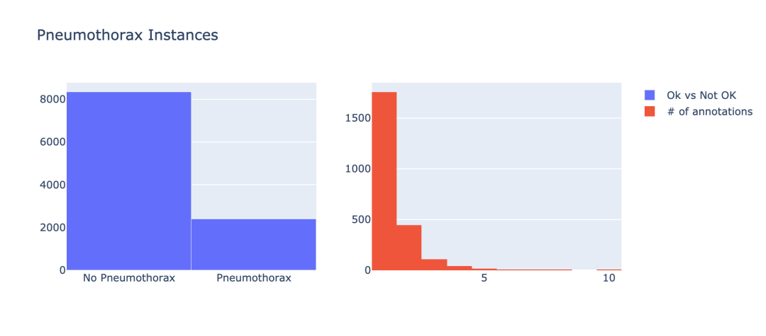
接下来，我们需要查看患有气胸的数据和未患有气胸的数据的分布情况。

nok_count = train_metadata_df['has_pneumothorax'].sum()
ok_count = len(train_metadata_df) - nok_count
x = ['No Pneumothorax','Pneumothorax']
y = [ok_count, nok_count]
trace0 = Bar(x=x, y=y, name = 'Ok vs Not OK')
nok_encoded_pixels_count = train_metadata_df[train_metadata_df['has_pneumothorax']==1]['encoded_pixels_count'].values
trace1 = Histogram(x=nok_encoded_pixels_count, name='# of annotations')
fig = subplots.make_subplots(rows=1, cols=2)
fig.append_trace(trace0, 1, 1)
fig.append_trace(trace1, 1, 2)
fig['layout'].update(height=400, width=900, title='Pneumothorax Instances')
iplot(fig)

结果如图示：

3.3 气胸患者的年龄分布

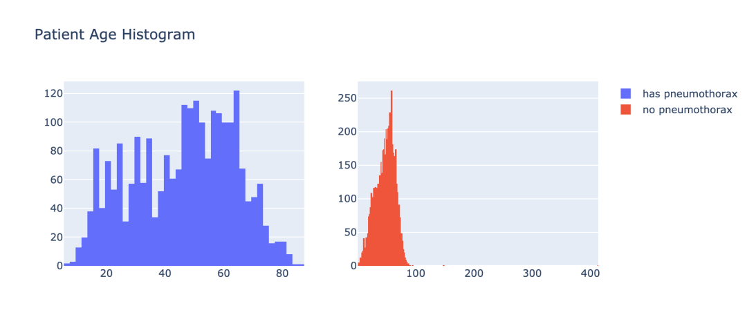
在让我们通过年龄的角度来看下气胸患者的分布情况。

train_male_df = train_metadata_df[train_metadata_df['patient_sex']=='M']
train_female_df = train_metadata_df[train_metadata_df['patient_sex']=='F']

pneumo_pat_age = train_metadata_df[train_metadata_df['has_pneumothorax']==1]['patient_age'].values
no_pneumo_pat_age = train_metadata_df[train_metadata_df['has_pneumothorax']==0]['patient_age'].values

pneumothorax = Histogram(x=pneumo_pat_age, name='has pneumothorax')
no_pneumothorax = Histogram(x=no_pneumo_pat_age, name='no pneumothorax')
fig = subplots.make_subplots(rows=1, cols=2)
fig.append_trace(pneumothorax, 1, 1)
fig.append_trace(no_pneumothorax, 1, 2)
fig['layout'].update(height=400, width=900, title='Patient Age Histogram')
iplot(fig)

结果如图示：

3.4 气胸患者的性别分布

让我们通过性别的角度来查看下气胸患者的分布情况。

train_male_df = train_metadata_df[train_metadata_df['patient_sex']=='M']
train_female_df = train_metadata_df[train_metadata_df['patient_sex']=='F']
male_ok_count = len(train_male_df[train_male_df['has_pneumothorax']==0])
female_ok_count = len(train_female_df[train_female_df['has_pneumothorax']==0])
male_nok_count = len(train_male_df[train_male_df['has_pneumothorax']==1])
female_nok_count = len(train_female_df[train_female_df['has_pneumothorax']==1])
ok = Bar(x=['male', 'female'], y=[male_ok_count, female_ok_count], name='no pneumothorax')
nok = Bar(x=['male', 'female'], y=[male_nok_count, female_nok_count], name='has pneumothorax')

data = [ok, nok]
layout = Layout(barmode='stack', height=400)

fig = Figure(data=data, layout=layout)
iplot(fig, filename='stacked-bar')

结果如图示：

m_pneumo_labels = ['no pneumothorax','has pneumothorax']
f_pneumo_labels = ['no pneumothorax','has pneumothorax']
m_pneumo_values = [male_ok_count, male_nok_count]
f_pneumo_values = [female_ok_count, female_nok_count]
colors = ['#FEBFB3', '#E1396C']

fig = {
  "data": [
    {
      "values": m_pneumo_values,
      "labels": m_pneumo_labels,
      "domain": {"column": 0},
      "name": "Male",
      "hoverinfo":"label+percent",
      "hole": .4,
      "type": "pie"
    },
    {
      "values": f_pneumo_values,
      "labels": f_pneumo_labels,
      "textposition":"inside",
      "domain": {"column": 1},
      "name": "Female",
      "hoverinfo":"label+percent",
      "hole": .4,
      "type": "pie"
    }],

结果如图示：

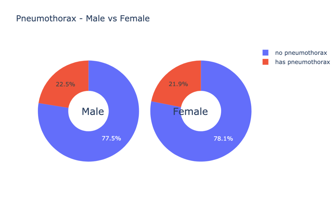
数据可视化是分析数据的一种重要手段，通过上面几个例子，给大家展示了一些比较常用的数据可视化的方法。

第四步：数据清洗

下面我们来看下，我们的数据内是否含有无效的数据，无效的数据指的是我们胸片图片跟 mask 上不一致，也可以说我们的胸片并未被标记标签。

在第二步骤中有说明 mask 是以 RLE 编码的，如果是气胸患者，那么他的 RLE 数据段是有值的，如果他不是我们是以 -1 来标示。

在刚才读取 dcm 的函数里，我们把 EncodedPixels 字段的数据长度给记录下来，正常的数据长度必须是 >0 。

因此我们可以简单的查看下记录 EncodedPixels 长度的 encoded_pixels_count 字段中值是否为 0，来简单的过滤下我们的非正常数据。

missing_vals = train_metadata_df[train_metadata_df['encoded_pixels_count']==0]['encoded_pixels_count'].count()
print("Number of x-rays with missing masks: {}".format(missing_vals))

我们可以看到，有37份数据是没有标签，后面我们需要删除它们。

第五步：准备训练数据

我们先来定义一些我们将要使用到的一些常数。

# 图像大小
img_size = 256
# batch size
batch_size = 16
# 卷积kernel的大小
k_size = 3
# 训练数据跟验证数据的分割比例
val_size = .1

5.1 数据生成类

class DataGenerator(tf.keras.utils.Sequence):
    def __init__(self, file_path_list, labels, batch_size=32,
                 img_size=256, channels=1, shuffle=True, augmentations=None):
        self.file_path_list = file_path_list
        self.labels = labels
        self.batch_size = batch_size
        self.img_size = img_size
        self.channels = channels
        self.shuffle = shuffle
        self.augment = augmentations
        self.on_epoch_end()

    def __len__(self):
        return int(np.floor(len(self.file_path_list)) / self.batch_size)

    def __getitem__(self, index):
        indexes = self.indexes[index*self.batch_size:(index+1)*self.batch_size]
        file_path_list_temp = [self.file_path_list[k] for k in indexes]
        X, y = self.__data_generation(file_path_list_temp)
        if self.augment is None:
            return X,np.array(y)/255
        else:
            im,mask = [],[]
            for x,y in zip(X,y):
                augmented = self.augment(image=x, mask=y)
                im.append(augmented['image'])
                mask.append(augmented['mask'])
            return np.array(im),np.array(mask)/255

5.2 数据增强

数据增强有助于提高数据的数量，因为你每做一次变换相当于得到了一张新的图片；

同时也能提高模型的泛化能力，因为你的数据分布相较于没做数据增强的数据的分布更加的广泛。

AUGMENTATIONS_TRAIN = Compose([
    HorizontalFlip(p=0.5),
    OneOf([
        RandomContrast(),
        RandomGamma(),
        RandomBrightness(),
         ], p=0.3),
    OneOf([
        ElasticTransform(alpha=120, sigma=120 * 0.05, alpha_affine=120 * 0.03),
        GridDistortion(),
        OpticalDistortion(distort_limit=2, shift_limit=0.5),
        ], p=0.3),
    RandomSizedCrop(min_max_height=(156, 256), height=img_size, width=img_size, p=0.25),
    ToFloat(max_value=1)
],p=1)

AUGMENTATIONS_VALIDATION = Compose([
    ToFloat(max_value=1)
],p=1)

第六步：定义模型

在图像分割中, 有很多模型都可以达到很好的效果. 今天我们选用的模型是 UNet 的变形。

使用tensorflow的keras接口定义我们的 ResUNet 。

    'batch normalization layer with an optinal activation layer'
    x = tf.keras.layers.BatchNormalization()(x)
    if act == True:
        x = tf.keras.layers.Activation('relu')(x)
    return x

def conv_block(x, filters, kernel_size=3, padding='same', strides=1):
    'convolutional layer which always uses the batch normalization layer'
    conv = bn_act(x)
    conv = Conv2D(filters, kernel_size, padding=padding, strides=strides)(conv)
    return conv

def stem(x, filters, kernel_size=3, padding='same', strides=1):
    conv = Conv2D(filters, kernel_size, padding=padding, strides=strides)(x)
    conv = conv_block(conv, filters, kernel_size, padding, strides)
    shortcut = Conv2D(filters, kernel_size=1, padding=padding, strides=strides)(x)
    shortcut = bn_act(shortcut, act=False)
    output = Add()([conv, shortcut])
    return output

def residual_block(x, filters, kernel_size=3, padding='same', strides=1):
    res = conv_block(x, filters, k_size, padding, strides)
    res = conv_block(res, filters, k_size, padding, 1)
    shortcut = Conv2D(filters, kernel_size, padding=padding, strides=strides)(x)
    shortcut = bn_act(shortcut, act=False)
    output = Add()([shortcut, res])
    return output

定义我们的模型对象，并且 Summary 一下看下模型的细节。

model = ResUNet(img_size)
model.compile(optimizer="adam", loss=bce_dice_loss, metrics=[iou_metric])
model.summary()

第七步：开始训练

epochs=70
callback = LearningRateCallbackBuilder(nb_epochs=epochs,nb_snapshots=1,init_lr=1e-3)
history = model.fit_generator(generator=training_generator, validation_data=validation_generator, callbacks=callback.get_callbacks(), epochs=epochs, verbose=2)

第八步：训练结果查看

# 模型的IoU
plt.figure(figsize=(16,4))
plt.subplot(1,2,1)
plt.plot(history.history['iou_metric'][1:])
plt.plot(history.history['val_iou_metric'][1:])

# 模型的loss
plt.subplot(1,2,2)
plt.plot(history.history['loss'][1:])
plt.plot(history.history['val_loss'][1:])
plt.ylabel('val_loss')

训练数据的 loss 跟验证数据的 loss 的走势对比，训练数据的 IoU 跟验证数据的 IoU 的走势对比。

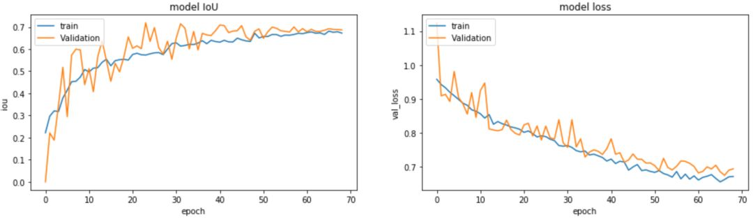
通过上面两个走势我们可以看出，我们的模型在不断的收敛的。

count = 0
for i in range(0,30):
    if count <= 15:
        x, y = validation_generator.__getitem__(i)
        predictions = model.predict(x)
        for idx, val in enumerate(x):
            if y[idx].sum() > 0 and count <= 15:
                img = np.reshape(x[idx]* 255, (img_size, img_size))
                mask = np.reshape(y[idx]* 255, (img_size, img_size))
                pred = np.reshape(predictions[idx], (img_size, img_size))
                pred = pred > 0.5
                pred = pred * 255
                plot_train(img, mask, pred)
                count += 1

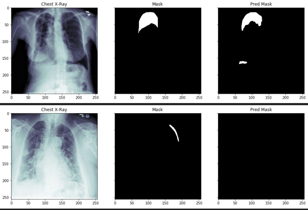
通过上述图片，我们可以看到气胸的阴影面积和位置，已经被分离出来了。但是，某些参数还需要进一步的调整。

大家可以登陆矩池云国内领先的GPU云共享平台，选择demo镜像，进行该气胸分割案例尝试。