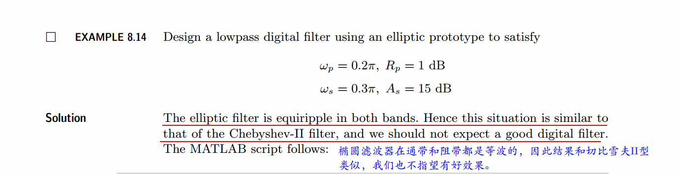
《DSP using MATLAB》示例Example 8.14

%% ------------------------------------------------------------------------
%%            Output Info about this m-file
fprintf('\n***********************************************************\n');
fprintf('        <DSP using MATLAB> Exameple 8.14 \n\n');

time_stamp = datestr(now, 31);
[wkd1, wkd2] = weekday(today, 'long');
fprintf('      Now is %20s, and it is %8s  \n\n', time_stamp, wkd2);
%% ------------------------------------------------------------------------

% Digital Filter Specifications:
wp = 0.2*pi;                 % digital passband freq in rad
ws = 0.3*pi;                 % digital stopband freq in rad
Rp = 1;                      % passband ripple in dB
As = 15;                     % stopband attenuation in dB

% Analog prototype specifications: Inverse Mapping for frequencies
T = 1;                       % set T = 1
OmegaP = wp/T;               % prototype passband freq
OmegaS = ws/T;               % prototype stopband freq

% Analog Elliptic Prototype Filter Calculation:
[cs, ds] = afd_elip(OmegaP, OmegaS, Rp, As);

% Impulse Invariance Transformation:
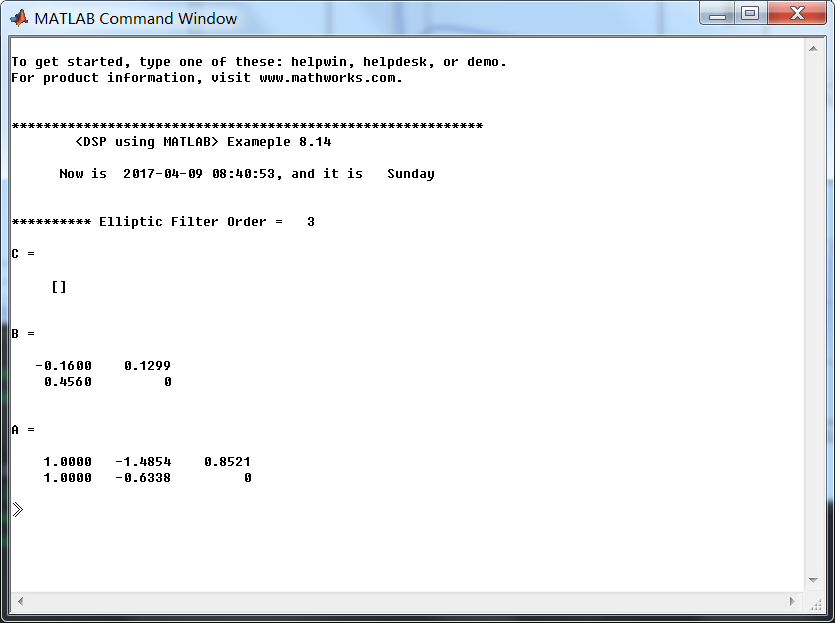
[b, a] = imp_invr(cs, ds, T); [C, B, A] = dir2par(b, a)

% Calculation of Frequency Response:
[db, mag, pha, grd, ww] = freqz_m(b, a);

%% -----------------------------------------------------------------
%%                             Plot
%% -----------------------------------------------------------------  

figure('NumberTitle', 'off', 'Name', 'Exameple 8.14')
set(gcf,'Color','white');
M = 1;                          % Omega max

subplot(2,2,1); plot(ww/pi, mag); axis([0, M, 0, 1.2]); grid on;
xlabel(' frequency in \pi units'); ylabel('|H|'); title('Magnitude Response');
set(gca, 'XTickMode', 'manual', 'XTick', [0, 0.2, 0.3, M]);
set(gca, 'YTickMode', 'manual', 'YTick', [0, 0.1778, 0.8913, 1]);

subplot(2,2,2); plot(ww/pi, pha/pi); axis([0, M, -1.1, 1.1]); grid on;
xlabel('frequency in \pi nuits'); ylabel('radians in \pi units'); title('Phase Response');
set(gca, 'XTickMode', 'manual', 'XTick', [0, 0.2, 0.3, M]);
set(gca, 'YTickMode', 'manual', 'YTick', [-1:1:1]);

subplot(2,2,3); plot(ww/pi, db); axis([0, M, -30, 10]); grid on;
xlabel('frequency in \pi units'); ylabel('Decibels'); title('Magnitude in dB ');
set(gca, 'XTickMode', 'manual', 'XTick', [0, 0.2, 0.3, M]);
set(gca, 'YTickMode', 'manual', 'YTick', [-30, -15, -1, 0]);

subplot(2,2,4); plot(ww/pi, grd); axis([0, M, 0, 20]); grid on;
xlabel('frequency in \pi units'); ylabel('Samples'); title('Group Delay');
set(gca, 'XTickMode', 'manual', 'XTick', [0, 0.2, 0.3, M]);
set(gca, 'YTickMode', 'manual', 'YTick', [0:5:20]);

　　运行结果：

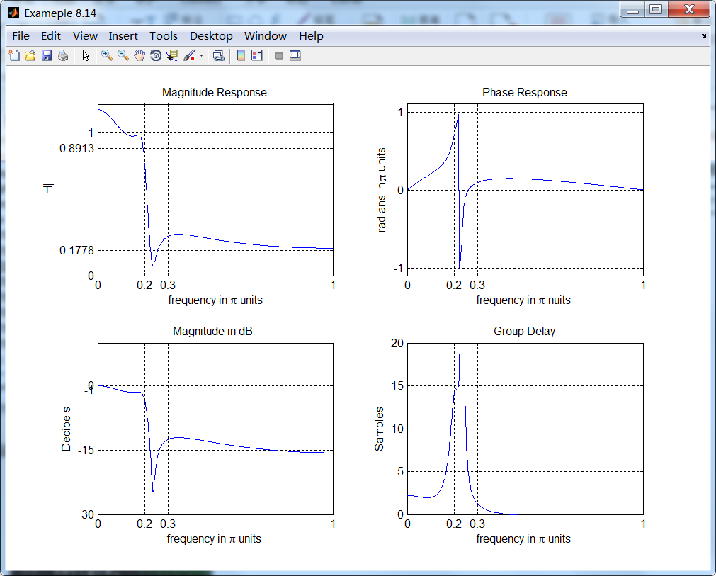
从图上看出，脉冲不变设计方法又失败了。

脉冲不变方法的优点是稳定的设计，频率Ω和ω是线性相关的。但是缺点是模拟频率响应中有一些假频，某些情况下假频是无法容忍的。

结论：该设计方法仅当模拟滤波器是带限到低通或带通的情况（阻带中没有振荡）。