
沉淀再出发:使用python进行机器学习
沉淀再出发:使用python进行机器学习
一、前言
使用python进行学习运算和机器学习是非常方便的,因为其中有很多的库函数可以使用,同样的python自身语言的特点也非常利于程序的编写和使用。
二、几个简单的例子
2.1、使用python实现KNN算法
 #########################################

 # kNN: k Nearest Neighbors

 # Input:      newInput: vector to compare to existing dataset (1xN)

 #             dataSet:  size m data set of known vectors (NxM)

 #             labels:     data set labels (1xM vector)

 #             k:         number of neighbors to use for comparison

 # Output:     the most popular class label

 #########################################

 from numpy import *

 import operator

 # create a dataset which contains 4 samples with 2 classes

 def createDataSet():

     # create a matrix: each row as a sample

     group = array([[1.0, 0.9], [1.0, 1.0], [0.1, 0.2], [0.0, 0.1]])

     labels = ['A', 'A', 'B', 'B'] # four samples and two classes

     return group, labels

 # classify using kNN

 def kNNClassify(newInput, dataSet, labels, k):

     numSamples = dataSet.shape[0] # shape[0] stands for the num of row

     ## step 1: calculate Euclidean distance

     # tile(A, reps): Construct an array by repeating A reps times

     # the following copy numSamples rows for dataSet

     diff = tile(newInput, (numSamples, 1)) - dataSet # Subtract element-wise

     squaredDiff = diff ** 2 # squared for the subtract

     squaredDist = sum(squaredDiff, axis = 1) # sum is performed by row

     distance = squaredDist ** 0.5

     ## step 2: sort the distance

     # argsort() returns the indices that would sort an array in a ascending order

     sortedDistIndices = argsort(distance)

     classCount = {} # define a dictionary (can be append element)

     for i in range(k):

         ## step 3: choose the min k distance

         voteLabel = labels[sortedDistIndices[i]]

         ## step 4: count the times labels occur

         # when the key voteLabel is not in dictionary classCount, get()

         # will return 0

         classCount[voteLabel] = classCount.get(voteLabel, 0) + 1

     ## step 5: the max voted class will return

     maxCount = 0

     for key, value in classCount.items():

         if value > maxCount:

             maxCount = value

             maxIndex = key

     return maxIndex
测试文件:
 import knn

 from numpy import *

 dataSet, labels = knn.createDataSet()

 testX = array([1.2, 1.0])

 k = 3

 k = 3

 outputLabel = knn.kNNClassify(testX, dataSet, labels, 3)

 print ("Your input is:", testX, "and classified to class: ", outputLabel)

 testX = array([0.1, 0.3])

 outputLabel = knn.kNNClassify(testX, dataSet, labels, 3)

 print ("Your input is:", testX, "and classified to class: ", outputLabel)
其中knn的思路非常简单,就是在某一个范围内观察距离该需要归类的样本的所有样本之中,那一个种类的样本数目最多,通过对附近的K个样本的寻找来进行分类。

2.2、使用scikit-learn库进行机器学习
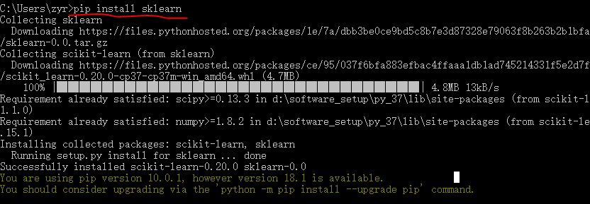
 #!usr/bin/env python

 # coding:utf-8

 import sys

 import os

 import time

 from sklearn import metrics

 import numpy as np

 import pickle

 # import imp

 # imp.reload(sys)

 # Multinomial Naive Bayes Classifier

 def naive_bayes_classifier(train_x, train_y):

     from sklearn.naive_bayes import MultinomialNB

     model = MultinomialNB(alpha=0.01)

     model.fit(train_x, train_y)

     return model

 # KNN Classifier

 def knn_classifier(train_x, train_y):

     from sklearn.neighbors import KNeighborsClassifier

     model = KNeighborsClassifier()

     model.fit(train_x, train_y)

     return model

 # Logistic Regression Classifier

 def logistic_regression_classifier(train_x, train_y):

     from sklearn.linear_model import LogisticRegression

     model = LogisticRegression(penalty='l2')

     model.fit(train_x, train_y)

     return model

 # Random Forest Classifier

 def random_forest_classifier(train_x, train_y):

     from sklearn.ensemble import RandomForestClassifier

     model = RandomForestClassifier(n_estimators=8)

     model.fit(train_x, train_y)

     return model

 # Decision Tree Classifier

 def decision_tree_classifier(train_x, train_y):

     from sklearn import tree

     model = tree.DecisionTreeClassifier()

     model.fit(train_x, train_y)

     return model

 # GBDT(Gradient Boosting Decision Tree) Classifier

 def gradient_boosting_classifier(train_x, train_y):

     from sklearn.ensemble import GradientBoostingClassifier

     model = GradientBoostingClassifier(n_estimators=200)

     model.fit(train_x, train_y)

     return model

 # SVM Classifier

 def svm_classifier(train_x, train_y):

     from sklearn.svm import SVC

     model = SVC(kernel='rbf', probability=True)

     model.fit(train_x, train_y)

     return model

 # SVM Classifier using cross validation

 def svm_cross_validation(train_x, train_y):

     from sklearn.grid_search import GridSearchCV

     from sklearn.svm import SVC

     model = SVC(kernel='rbf', probability=True)

     param_grid = {'C': [1e-3, 1e-2, 1e-1, 1, 10, 100, 1000], 'gamma': [0.001, 0.0001]}

     grid_search = GridSearchCV(model, param_grid, n_jobs = 1, verbose=1)

     grid_search.fit(train_x, train_y)

     best_parameters = grid_search.best_estimator_.get_params()

     for para, val in best_parameters.items():

         print (para, val)

     model = SVC(kernel='rbf', C=best_parameters['C'], gamma=best_parameters['gamma'], probability=True)

     model.fit(train_x, train_y)

     return model

 def read_data(data_file):

     import gzip

     f = gzip.open(data_file, "rb")

     train, val, test = pickle.load(f,encoding='bytes')

     f.close()

     train_x = train[0]

     train_y = train[1]

     test_x = test[0]

     test_y = test[1]

     return train_x, train_y, test_x, test_y

 if __name__ == '__main__':

     data_file = "mnist.pkl.gz"

     thresh = 0.5

     model_save_file = None

     model_save = {}

     test_classifiers = ['NB', 'KNN', 'LR', 'RF', 'DT', 'SVM', 'GBDT']

     classifiers = {'NB':naive_bayes_classifier,

                   'KNN':knn_classifier,

                    'LR':logistic_regression_classifier,

                    'RF':random_forest_classifier,

                    'DT':decision_tree_classifier,

                   'SVM':svm_classifier,

                 'SVMCV':svm_cross_validation,

                  'GBDT':gradient_boosting_classifier

     }

     print ('reading training and testing data...')

     train_x, train_y, test_x, test_y = read_data(data_file)

     num_train, num_feat = train_x.shape

     num_test, num_feat = test_x.shape

     is_binary_class = (len(np.unique(train_y)) == 2)

     print ('******************** Data Info *********************')

     print ('#training data: %d, #testing_data: %d, dimension: %d' % (num_train, num_test, num_feat))

     for classifier in test_classifiers:

         print ('******************* %s ********************' % classifier)

         start_time = time.time()

         model = classifiers[classifier](train_x, train_y)

         print ('training took %fs!' % (time.time() - start_time))

         predict = model.predict(test_x)

         if model_save_file != None:

             model_save[classifier] = model

         if is_binary_class:

             precision = metrics.precision_score(test_y, predict)

             recall = metrics.recall_score(test_y, predict)

             print ('precision: %.2f%%, recall: %.2f%%' % (100 * precision, 100 * recall))

         accuracy = metrics.accuracy_score(test_y, predict)

         print ('accuracy: %.2f%%' % (100 * accuracy) )

     if model_save_file != None:

         pickle.dump(model_save, open(model_save_file, 'wb'))
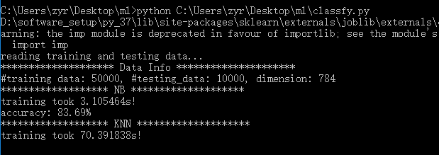
其中数据集使用的minst数据集。
2.3、sklearn的使用
     Supervised Learning

         Classification

         Regression

         Measuring performance

     Unsupervised Learning

         Clustering

         Dimensionality Reduction

         Density Estimation

     Evaluation of Learning Models

     Choosing the right algorithm for your dataset
2.3.1、分类任务(随机梯度下降(SGD)算法)
 >>> import matplotlib.pyplot as plt

 >>> plt.style.use('seaborn')

 >>> from fig_code import plot_sgd_separator

 >>> plot_sgd_separator()

 >>> plt.show()
其中sgd_separator.py:
 import numpy as np

 import matplotlib.pyplot as plt

 from sklearn.linear_model import SGDClassifier

 from sklearn.datasets.samples_generator import make_blobs

 def plot_sgd_separator():

     # we create 50 separable points

     X, Y = make_blobs(n_samples=50, centers=2,

                       random_state=0, cluster_std=0.60)

     # fit the model

     clf = SGDClassifier(loss="hinge", alpha=0.01,

                         max_iter=200, fit_intercept=True)

     clf.fit(X, Y)

     # plot the line, the points, and the nearest vectors to the plane

     xx = np.linspace(-1, 5, 10)

     yy = np.linspace(-1, 5, 10)

     X1, X2 = np.meshgrid(xx, yy)

     Z = np.empty(X1.shape)

     for (i, j), val in np.ndenumerate(X1):

         x1 = val

         x2 = X2[i, j]

         p = clf.decision_function(np.array([x1, x2]).reshape(1, -1))

         Z[i, j] = p[0]

     levels = [-1.0, 0.0, 1.0]

     linestyles = ['dashed', 'solid', 'dashed']

     colors = 'k'

     ax = plt.axes()

     ax.contour(X1, X2, Z, levels, colors=colors, linestyles=linestyles)

     ax.scatter(X[:, 0], X[:, 1], c=Y, cmap=plt.cm.Paired)

     ax.axis('tight')

 if __name__ == '__main__':

     plot_sgd_separator()

     plt.show()

2.3.2、线性回归任务
@1、linear_regression.py:
 import numpy as np

 import matplotlib.pyplot as plt

 from sklearn.linear_model import LinearRegression

 def plot_linear_regression():

     a = 0.5

     b = 1.0

     # x from 0 to 10

     x = 30 * np.random.random(20)

     # y = a*x + b with noise

     y = a * x + b + np.random.normal(size=x.shape)

     # create a linear regression classifier

     clf = LinearRegression()

     clf.fit(x[:, None], y)

     # predict y from the data

     x_new = np.linspace(0, 30, 100)

     y_new = clf.predict(x_new[:, None])

     # plot the results

     ax = plt.axes()

     ax.scatter(x, y)

     ax.plot(x_new, y_new)

     ax.set_xlabel('x')

     ax.set_ylabel('y')

     ax.axis('tight')

 if __name__ == '__main__':

     plot_linear_regression()

     plt.show()
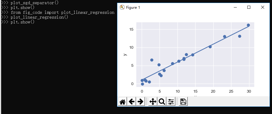
导入上面的程序并使用:
 >>> from fig_code import plot_linear_regression

 >>> plot_linear_regression()

 >>> plt.show()
@2、接下来我们自己生成数据并进行拟合:
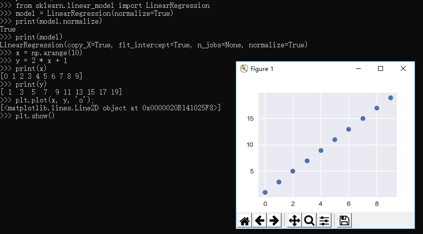
生成模型:
 >>> from sklearn.linear_model import LinearRegression

 >>> model = LinearRegression(normalize=True)

 >>> print(model.normalize)

 True

 >>> print(model)

 LinearRegression(copy_X=True, fit_intercept=True, n_jobs=None, normalize=True)
生成数据:
 >>> x = np.arange(10)

 >>> y = 2 * x + 1

 >>> print(x)

 [0 1 2 3 4 5 6 7 8 9]

 >>> print(y)

 [ 1  3  5  7  9 11 13 15 17 19]

 >>> plt.plot(x, y, 'o');

 [<matplotlib.lines.Line2D object at 0x0000020B141025F8>]

 >>> plt.show()

 >>>
进行拟合:
 >>> X = x[:, np.newaxis]

 >>> print(X)

 [[0]

  [1]

  [2]

  [3]

  [4]

  [5]

  [6]

  [7]

  [8]

  [9]]

 >>> print(y)

 [ 1  3  5  7  9 11 13 15 17 19]

 >>> model.fit(X, y)

 LinearRegression(copy_X=True, fit_intercept=True, n_jobs=None, normalize=True)

 >>> print(model.coef_)

 [2.]

 >>> print(model.intercept_)

 0.9999999999999982

 >>>
可以看到斜率和截距确实是我们期望的。
2.3.3、Iris Dataset的简单样例
 >>> from sklearn.datasets import load_iris

 >>> iris = load_iris()

 >>> iris.keys()

 dict_keys(['data', 'target', 'target_names', 'DESCR', 'feature_names', 'filename'])

 >>> n_samples, n_features = iris.data.shape

 >>> print((n_samples, n_features))

 (150, 4)

 >>> print(iris.data[0])

 [5.1 3.5 1.4 0.2]

 >>> print(iris.data.shape)

 (150, 4)

 >>> print(iris.target.shape)

 (150,)

 >>> print(iris.target)

 [0 0 0 0 0 0 0 0 0 0 0 0 0 0 0 0 0 0 0 0 0 0 0 0 0 0 0 0 0 0 0 0 0 0 0 0 0

  0 0 0 0 0 0 0 0 0 0 0 0 0 1 1 1 1 1 1 1 1 1 1 1 1 1 1 1 1 1 1 1 1 1 1 1 1

  1 1 1 1 1 1 1 1 1 1 1 1 1 1 1 1 1 1 1 1 1 1 1 1 1 1 2 2 2 2 2 2 2 2 2 2 2

  2 2 2 2 2 2 2 2 2 2 2 2 2 2 2 2 2 2 2 2 2 2 2 2 2 2 2 2 2 2 2 2 2 2 2 2 2

  2 2]

 >>> print(iris.target_names)

 ['setosa' 'versicolor' 'virginica']

 >>> import numpy as np

 >>> import matplotlib.pyplot as plt

 >>> x_index = 0

 >>> y_index = 1

 >>> formatter = plt.FuncFormatter(lambda i, *args: iris.target_names[int(i)])

 >>> plt.scatter(iris.data[:, x_index], iris.data[:, y_index],

 ...             c=iris.target, cmap=plt.cm.get_cmap('RdYlBu', 3))

 <matplotlib.collections.PathCollection object at 0x0000020B0BDE89B0>

 >>> plt.colorbar(ticks=[0, 1, 2], format=formatter)

 <matplotlib.colorbar.Colorbar object at 0x0000020B0AFC8A58>

 >>> plt.clim(-0.5, 2.5)

 >>> plt.xlabel(iris.feature_names[x_index])

 Text(0.5, 0, 'sepal length (cm)')

 >>> plt.ylabel(iris.feature_names[y_index]);

 Text(0, 0.5, 'sepal width (cm)')

 >>> plt.show()

 >>>
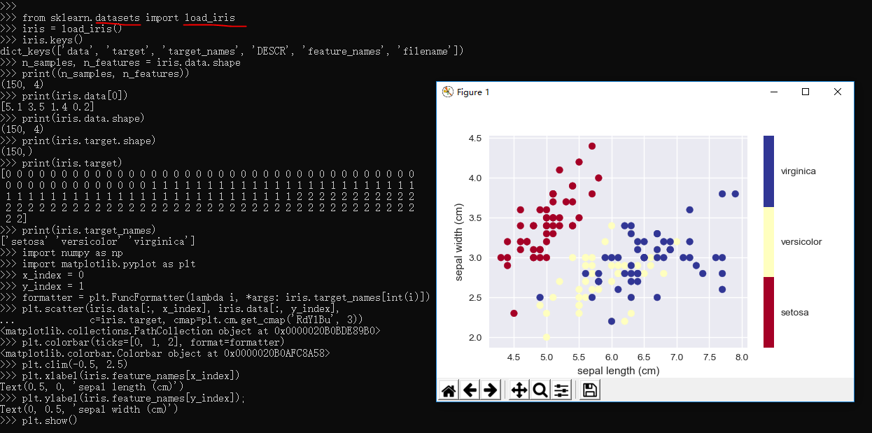
2.3.4、knn分类器
 """

 Small helpers for code that is not shown in the notebooks

 """

 from sklearn import neighbors, datasets, linear_model

 import pylab as pl

 import numpy as np

 from matplotlib.colors import ListedColormap

 # Create color maps for 3-class classification problem, as with iris

 cmap_light = ListedColormap(['#FFAAAA', '#AAFFAA', '#AAAAFF'])

 cmap_bold = ListedColormap(['#FF0000', '#00FF00', '#0000FF'])

 def plot_iris_knn():

     iris = datasets.load_iris()

     X = iris.data[:, :2]  # we only take the first two features. We could

                         # avoid this ugly slicing by using a two-dim dataset

     y = iris.target

     knn = neighbors.KNeighborsClassifier(n_neighbors=3)

     knn.fit(X, y)

     x_min, x_max = X[:, 0].min() - .1, X[:, 0].max() + .1

     y_min, y_max = X[:, 1].min() - .1, X[:, 1].max() + .1

     xx, yy = np.meshgrid(np.linspace(x_min, x_max, 100),

                          np.linspace(y_min, y_max, 100))

     Z = knn.predict(np.c_[xx.ravel(), yy.ravel()])

     # Put the result into a color plot

     Z = Z.reshape(xx.shape)

     pl.figure()

     pl.pcolormesh(xx, yy, Z, cmap=cmap_light)

     # Plot also the training points

     pl.scatter(X[:, 0], X[:, 1], c=y, cmap=cmap_bold)

     pl.xlabel('sepal length (cm)')

     pl.ylabel('sepal width (cm)')

     pl.axis('tight')

 def plot_polynomial_regression():

     rng = np.random.RandomState(0)

     x = 2*rng.rand(100) - 1

     f = lambda t: 1.2 * t**2 + .1 * t**3 - .4 * t **5 - .5 * t ** 9

     y = f(x) + .4 * rng.normal(size=100)

     x_test = np.linspace(-1, 1, 100)

     pl.figure()

     pl.scatter(x, y, s=4)

     X = np.array([x**i for i in range(5)]).T

     X_test = np.array([x_test**i for i in range(5)]).T

     regr = linear_model.LinearRegression()

     regr.fit(X, y)

     pl.plot(x_test, regr.predict(X_test), label='4th order')

     X = np.array([x**i for i in range(10)]).T

     X_test = np.array([x_test**i for i in range(10)]).T

     regr = linear_model.LinearRegression()

     regr.fit(X, y)

     pl.plot(x_test, regr.predict(X_test), label='9th order')

     pl.legend(loc='best')

     pl.axis('tight')

     pl.title('Fitting a 4th and a 9th order polynomial')

     pl.figure()

     pl.scatter(x, y, s=4)

     pl.plot(x_test, f(x_test), label="truth")

     pl.axis('tight')

     pl.title('Ground truth (9th order polynomial)')
引用上面的包:
 >>> from sklearn import neighbors, datasets

 >>> iris = datasets.load_iris()

 >>> X, y = iris.data, iris.target

 >>> knn = neighbors.KNeighborsClassifier(n_neighbors=5)

 >>> knn.fit(X, y)

 KNeighborsClassifier(algorithm='auto', leaf_size=30, metric='minkowski',

            metric_params=None, n_jobs=None, n_neighbors=5, p=2,

            weights='uniform')

 >>> result = knn.predict([[3, 5, 4, 2],])

 >>> print(iris.target_names[result])

 ['versicolor']

 >>> knn.predict_proba([[3, 5, 4, 2],])

 array([[0. , 0.8, 0.2]])

 >>> from fig_code import plot_iris_knn

 >>> plot_iris_knn()

 >>> plt.show()

 >>>
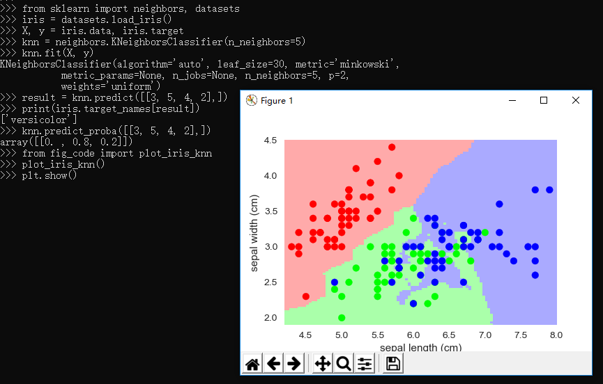
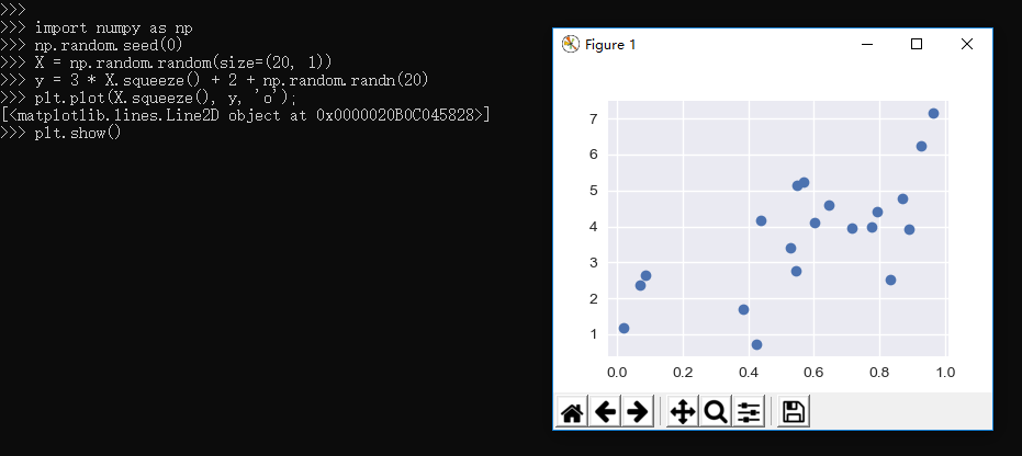
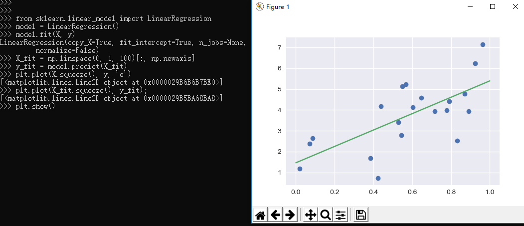
2.3.5、Regression Example
 >>> import numpy as np

 >>> np.random.seed(0)

 >>> X = np.random.random(size=(20, 1))

 >>> y = 3 * X.squeeze() + 2 + np.random.randn(20)

 >>> plt.plot(X.squeeze(), y, 'o');

 [<matplotlib.lines.Line2D object at 0x0000020B0C045828>]

 >>> plt.show()
 >>>

 >>> from sklearn.linear_model import LinearRegression

 >>> model = LinearRegression()

 >>> model.fit(X, y)

 LinearRegression(copy_X=True, fit_intercept=True, n_jobs=None,

          normalize=False)

 >>> X_fit = np.linspace(0, 1, 100)[:, np.newaxis]

 >>> y_fit = model.predict(X_fit)

 >>> plt.plot(X.squeeze(), y, 'o')

 [<matplotlib.lines.Line2D object at 0x0000029B6B6B7BE0>]

 >>> plt.plot(X_fit.squeeze(), y_fit);

 [<matplotlib.lines.Line2D object at 0x0000029B5BA68BA8>]

 >>> plt.show()
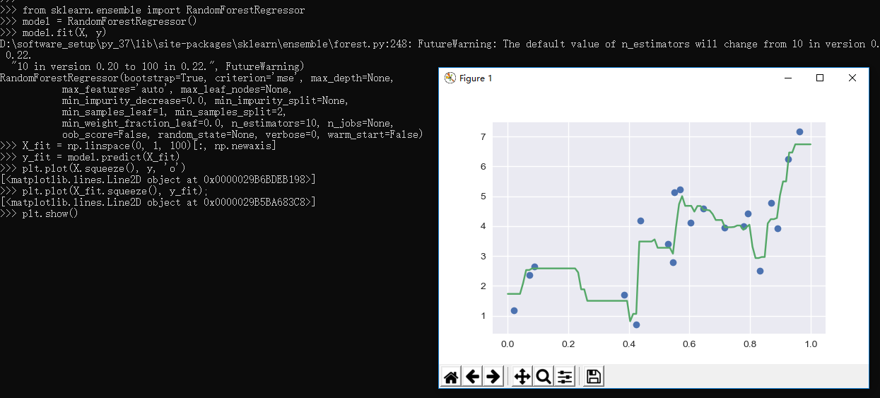
Scikit-learn also has some more sophisticated models, which can respond to finer features in the data::
 >>> from sklearn.ensemble import RandomForestRegressor

 >>> model = RandomForestRegressor()

 >>> model.fit(X, y)

 FutureWarning: The default value of n_estimators will change from 10 in version 0.20 to 100 in 0.22.

   "10 in version 0.20 to 100 in 0.22.", FutureWarning)

 RandomForestRegressor(bootstrap=True, criterion='mse', max_depth=None,

            max_features='auto', max_leaf_nodes=None,

            min_impurity_decrease=0.0, min_impurity_split=None,

            min_samples_leaf=1, min_samples_split=2,

            min_weight_fraction_leaf=0.0, n_estimators=10, n_jobs=None,

            oob_score=False, random_state=None, verbose=0, warm_start=False)

 >>> X_fit = np.linspace(0, 1, 100)[:, np.newaxis]

 >>> y_fit = model.predict(X_fit)

 >>> plt.plot(X.squeeze(), y, 'o')

 [<matplotlib.lines.Line2D object at 0x0000029B6BDEB198>]

 >>> plt.plot(X_fit.squeeze(), y_fit);

 [<matplotlib.lines.Line2D object at 0x0000029B5BA683C8>]

 >>> plt.show()

 >>>
2.3.6、Dimensionality Reduction: PCA
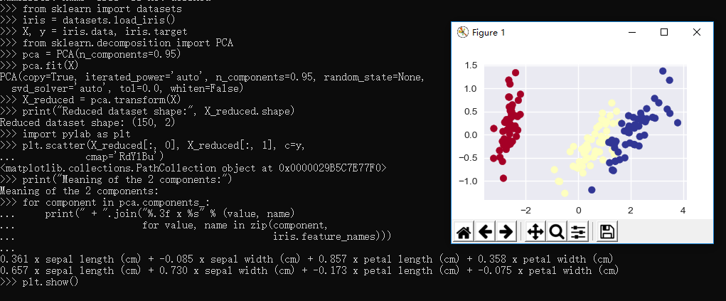
 >>> from sklearn import datasets

 >>> iris = datasets.load_iris()

 >>> X, y = iris.data, iris.target

 >>> from sklearn.decomposition import PCA

 >>> pca = PCA(n_components=0.95)

 >>> pca.fit(X)

 PCA(copy=True, iterated_power='auto', n_components=0.95, random_state=None,

   svd_solver='auto', tol=0.0, whiten=False)

 >>> X_reduced = pca.transform(X)

 >>> print("Reduced dataset shape:", X_reduced.shape)

 Reduced dataset shape: (150, 2)

 >>> import pylab as plt

 >>> plt.scatter(X_reduced[:, 0], X_reduced[:, 1], c=y,

 ...            cmap='RdYlBu')

 <matplotlib.collections.PathCollection object at 0x0000029B5C7E77F0>

 >>> print("Meaning of the 2 components:")

 Meaning of the 2 components:

 >>> for component in pca.components_:

 ...     print(" + ".join("%.3f x %s" % (value, name)

 ...                      for value, name in zip(component,

 ...                                             iris.feature_names)))

 ...

 0.361 x sepal length (cm) + -0.085 x sepal width (cm) + 0.857 x petal length (cm) + 0.358 x petal width (cm)

 0.657 x sepal length (cm) + 0.730 x sepal width (cm) + -0.173 x petal length (cm) + -0.075 x petal width (cm)

 >>> plt.show()

 >>>
2.3.7、Clustering: K-means
 >>> from sklearn.cluster import KMeans

 >>> k_means = KMeans(n_clusters=3, random_state=0) # Fixing the RNG in kmeans

 >>> k_means.fit(X)

 KMeans(algorithm='auto', copy_x=True, init='k-means++', max_iter=300,

     n_clusters=3, n_init=10, n_jobs=None, precompute_distances='auto',

     random_state=0, tol=0.0001, verbose=0)

 >>> y_pred = k_means.predict(X)

 >>> plt.scatter(X_reduced[:, 0], X_reduced[:, 1], c=y_pred,

 ...            cmap='RdYlBu');

 <matplotlib.collections.PathCollection object at 0x0000029B5C7456A0>

 >>> plt.show()

 >>>

2.4、sklearn的模型验证
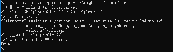
    An important piece of machine learning is model validation: that is, determining how well your model will generalize from the training data
to future unlabeled data. Let's look at an example using the nearest neighbor classifier. This is a very simple classifier:
    it simply stores all training data, and for any unknown quantity, simply returns the label of the closest training point.With the iris data,
    it very easily returns the correct prediction for each of the input points:
样例如下:
 >>> from sklearn.neighbors import KNeighborsClassifier

 >>> X, y = iris.data, iris.target

 >>> clf = KNeighborsClassifier(n_neighbors=1)

 >>> clf.fit(X, y)

 KNeighborsClassifier(algorithm='auto', leaf_size=30, metric='minkowski',

            metric_params=None, n_jobs=None, n_neighbors=1, p=2,

            weights='uniform')

 >>> y_pred = clf.predict(X)

 >>> print(np.all(y == y_pred))

 True

 >>>
A more useful way to look at the results is to view the confusion matrix, or the matrix showing the frequency of inputs and outputs:
>>> from sklearn.metrics import confusion_matrix

>>> print(confusion_matrix(y, y_pred))

[[50  0  0]

 [ 0 50  0]

 [ 0  0 50]]
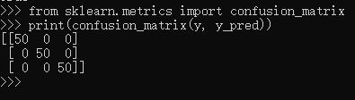
For each class, all 50 training samples are correctly identified. But this does not mean that our model is perfect! In particular, such a model generalizes extremely poorly to new data. We can simulate this by splitting our data into a training set and a testing set. Scikit-learn contains some convenient routines to do this:
>>> from sklearn.model_selection import train_test_split

>>> Xtrain, Xtest, ytrain, ytest = train_test_split(X, y)

>>> clf.fit(Xtrain, ytrain)

KNeighborsClassifier(algorithm='auto', leaf_size=30, metric='minkowski',

           metric_params=None, n_jobs=None, n_neighbors=1, p=2,

           weights='uniform')

>>> ypred = clf.predict(Xtest)

>>> print(confusion_matrix(ytest, ypred))

[[12  0  0]

 [ 0  6  0]

 [ 0  2 18]]
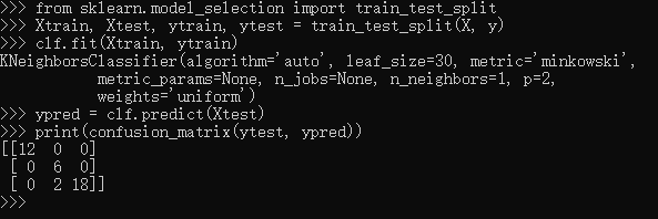
This paints a better picture of the true performance of our classifier: apparently there is some confusion between the second and third species, which we might anticipate given what we've seen of the data above.This is why it's extremely important to use a train/test split when evaluating your models.

沉淀再出发:使用python进行机器学习的更多相关文章
- 沉淀再出发:用python画各种图表
沉淀再出发:用python画各种图表 一.前言 最近需要用python来做一些统计和画图,因此做一些笔记. 二.python画各种图表 2.1.使用turtle来画图 import turtle as ...
- 沉淀,再出发:python中的pandas包
沉淀,再出发:python中的pandas包 一.前言 python中有很多的包,正是因为这些包工具才使得python能够如此强大,无论是在数据处理还是在web开发,python都发挥着重要的作用,下 ...
- 沉淀,再出发:python爬虫的再次思考
沉淀,再出发:python爬虫的再次思考 一.前言 之前笔者就写过python爬虫的相关文档,不过当时因为知识所限,理解和掌握的东西都非常的少,并且使用更多的是python2.x的版本的功能,现 ...
- 沉淀再出发:在python3中导入自定义的包
沉淀再出发:在python3中导入自定义的包 一.前言 在python中如果要使用自己的定义的包,还是有一些需要注意的事项的,这里简单记录一下. 二.在python3中导入自定义的包 2.1.什么是模 ...
- 沉淀再出发:mongodb的使用
沉淀再出发:mongodb的使用 一.前言 这是一篇很早就想写却一直到了现在才写的文章.作为NoSQL(not only sql)中出色的一种数据库,MongoDB的作用是非常大的,这种文档型数据库, ...
- 沉淀再出发:java中的equals()辨析
沉淀再出发:java中的equals()辨析 一.前言 关于java中的equals,我们可能非常奇怪,在Object中定义了这个函数,其他的很多类中都重载了它,导致了我们对于辨析其中的内涵有了混淆, ...
- 沉淀再出发:web服务器和应用服务器之间的区别和联系
沉淀再出发:web服务器和应用服务器之间的区别和联系 一.前言 关于后端,我们一般有三种服务器(当然还有文件服务器等),Web服务器,应用程序服务器和数据库服务器,其中前面两个的概念已经非常模糊了,但 ...
- 沉淀再出发:jetty的架构和本质
沉淀再出发:jetty的架构和本质 一.前言 我们在使用Tomcat的时候,总是会想到jetty,这两者的合理选用是和我们项目的类型和大小息息相关的,Tomcat属于比较重量级的容器,通过很多的容器层 ...
- 沉淀再出发:dubbo的基本原理和应用实例
沉淀再出发:dubbo的基本原理和应用实例 一.前言 阿里开发的dubbo作为服务治理的工具,在分布式开发中有着重要的意义,这里我们主要专注于dubbo的架构,基本原理以及在Windows下面开发出来 ...
随机推荐
- JavaScript设计模式-3.原型模式
<!DOCTYPE html> <html> <head> <meta charset="UTF-8"> <title> ...
- disable Nouveau kernel driver
nano /etc/modprobe.d/blacklist-nouveau.conf with the following contents: blacklist nouveau options n ...
- OpenLdap与BerkeleyDB安装过程
前段时间在看LDAP方面的东西,最近重装了Ubuntu之后开始在自己的机器上装一个OpenLDAP. 装的过程中还遇到不少问题,不过通过Google同学的帮忙,全部得到解决.下面装安装过程记录如下: ...
- InnoDB索引概述,二分查找法,平衡二叉树
索引是应用程序设计和开发的一个重要方面.如果索引太多,应用的性能可能会受到影响:如果索引太少,对查询性能又会产生影响.要找到一个合适的平衡点,这对应用的性能至关重要. 如果知道数据的使用,从一开始就应 ...
- BEA WebLogic平台下J2EE调优攻略--转载
BEA WebLogic平台下J2EE调优攻略 2008-06-25 作者:周海根 出处:网络 前 言 随着近来J2EE软件广泛地应用于各行各业,系统调优也越来越引起软件开发者和应用服务器提供 ...
- 以安全模式启动firefox
碰到firefox打开后一直没有响应,解决方法: 以安全模式打开
- java调用c/c++代码简单实现以及遇见的坑
以下内容均来自互联网,感谢你们的分享,我只是使用的时候看这方便,可以称呼我“搬运工” 如有不合适的地方请与我联系,我会及时改正 首先你可能会遇见以下错误 第一个错误是你在vs编译器没有选择使用rele ...
- JavaScript的柯里化函数
柯里化,或者说部分应用,是一种函数式编程的技术,对于熟悉以传统方式编写 JavaScript 代码的人来说可能会很费解.但如果使用得当,它可以使你的 JavaScript 函数更具可读性. 更具可读性 ...
- 批量删除SVN文件
开发过程中,有时需要将SVN目录中的SVN相关的信息去掉,有两种简单方法可以做到: 一,用SVN的export功能 二,将下面的这段文字写在.reg结尾的文本文件中,然后执行.这样你在每个文件夹右击的 ...
- layui——上传图片,并实现放大预览
一般上传文件后会返回文件的路径,然后存储到数据库,那么首先实现上传后的放大和删除功能 function uploadSmallPic() { var upload = layui.upload; up ...