论文解读（Debiased）《Debiased Contrastive Learning》

论文信息

论文标题：Debiased Contrastive Learning
论文作者：Ching-Yao Chuang, Joshua Robinson, Lin Yen-Chen, Antonio Torralba, Stefanie Jegelka
论文来源：2020, NeurIPS
论文地址：download
论文代码：download

1 Introduction

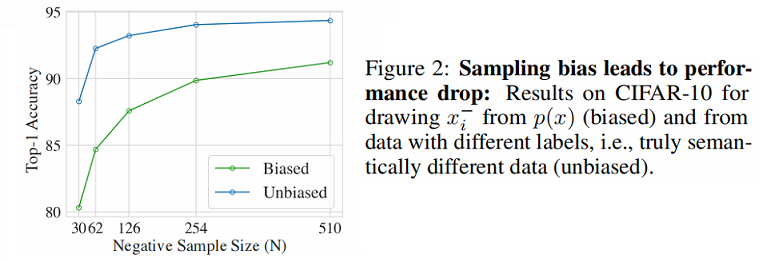
　　观察的结果：将拥有不同标签的样本作为负样本能显著提高性能。

　　对比学习思想：鼓励相似对 $\left(x, x^{+}\right)$ 的表示更接近，而不同对 $\left(x, x^{-}\right)$ 的表示更远：

　　　　$\mathbb{E}_{x, x^{+},\left\{x_{i}^{-}\right\}_{i=1}^{N}}\left[-\log \frac{e^{f(x)^{T} f\left(x^{+}\right)}}{e^{f(x)^{T} f\left(x^{+}\right)}+\sum\limits _{i=1}^{N} e^{f(x)^{T} f\left(x_{i}^{-}\right)}}\right] \quad\quad\quad(1)$

　　图解如下：

　　 

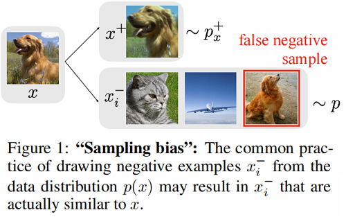
　　抽样偏差（sampling bias）：由于真正的标签或真正的语义相似性通常是不可用的，负对 $x^{-}$  通常从训练数据中抽取，这意味着 $x^{-}$  实际上可能和  $x$  相似。

　　$\text{Figure 2}$ 对比了不存在抽样偏差和存在抽样偏差的性能对比：

　　

　　设 $\mathcal{X}$ 上的数据分布 $p(x)$，代表语义意义的标签离散潜在类 $\mathcal{C}$，即相似的对 $\left(x, x^{+}\right)$ 具有相同的潜在类。用 $\rho(c)$ 表示类分布，得到联合分布 $p_{x, c}(x, c)=p(x \mid c) \rho(c)$。

　　设 $h: \mathcal{X} \rightarrow \mathcal{C}$ 是潜在类标签分配函数，然后  $p_{x}^{+}\left(x^{\prime}\right)=p\left(x^{\prime} \mid h\left(x^{\prime}\right)=h(x)\right) $ 中观察到的 $x^{\prime}$ 是 $x$ 的正对的概率，$p_{x}^{-}\left(x^{\prime}\right)=p\left(x^{\prime} \mid h\left(x^{\prime}\right) \neq h(x)\right)$ 中观察到的 $x^{\prime}$ 是 $x$ 的负对的概率。

　　假设类 $c$ 概率 $\rho(c)=\tau^{+}$ ，不是的概率为 $\tau^{-}=1-\tau^{+}$ 。

　　综上，对比损失函数可以优化为：

　　　　${\large L_{\text {Unbiased }}^{N}(f)=\mathbb{E}_{\substack{x \sim p, x^{+} \sim p_{-}^{+} \\ x_{i}^{-} \sim p_{x}^{-}}}\left[-\log \frac{e^{f(x)^{T} f\left(x^{+}\right)}}{e^{f(x)^{T} f\left(x^{+}\right)}+\frac{Q}{N} \sum\limits_{i=1}^{N} e^{f(x)^{T} f\left(x_{i}^{-}\right)}}\right]} \quad\quad\quad(2)$

　　其中，$Q $ 代表着权重参数。当 $Q=N$ 时，即标准的对比损失函数。

　　对有偏对比损失函数和无偏对比损失函数的分析：

　　Lemma 1. For any embedding $f$ and finite $N$, we have

　　　　${\large L_{\text {Biased }}^{N}(f) \geq L_{\text {Unbiased }}^{N}(f)+\mathbb{E}_{x \sim p}\left[0 \wedge \log \frac{\mathbb{E}_{x^{+} \sim p_{x}^{+}} \exp f(x)^{\top} f\left(x^{+}\right)}{\mathbb{E}_{x^{-} \sim p_{x}^{-}} \exp f(x)^{\top} f\left(x^{-}\right)}\right]-e^{3 / 2} \sqrt{\frac{\pi}{2 N}}} \quad\quad\quad(3)$

　　where $a \wedge b$ denotes the minimum of two real numbers $a$ and $b$.

　　Lemma 1 所带来的问题：

• • 无偏损失越小，第二项就越大，差距就越大；
  • 最小化 $L_{\text {Biased }}^{N}$ 的上界和最小化理想情况的 $L_{\text {Unbiased }}^{N}$ 所产生的潜在表示是不同的；

2 Method

　　我们首先将数据分布（data distribution）分解为【当从 $p(x)$ 中提取样本时，样本 $x_{i}^{-}$ 将来自与 $x$ 相同的类，概率为 $\tau^{+}$。】

　　　　$p\left(x^{\prime}\right)=\tau^{+} p_{x}^{+}\left(x^{\prime}\right)+\tau^{-} p_{x}^{-}\left(x^{\prime}\right)$

　　相应的

　　　　$p_{x}^{-}\left(x^{\prime}\right)=\left(p\left(x^{\prime}\right)-\tau^{+} p_{x}^{+}\left(x^{\prime}\right)\right) / \tau^{-}$

　　$\text{Eq.2}$ 的一种替代形式：

　　　　${\large \frac{1}{\left(\tau^{-}\right)^{N}} \sum\limits_{k=0}^{N}\left(\begin{array}{c}N \\k\end{array}\right)\left(-\tau^{+}\right)^{k} \mathbb{E}_{\substack{x p p, x^{+} \sim p_{x}^{+} \\\left\{x_{i}^{-}\right\}_{i=1}^{k} \sim p_{x}^{+} \\\left\{x_{i}^{-}\right\}_{i=k+1}^{N} \sim p}}\left[-\log \frac{e^{f(x)^{T} f\left(x^{+}\right)}}{e^{f(x)^{T} f\left(x^{+}\right)}+\sum\limits_{i=1}^{N} e^{f(x)^{T} f\left(x_{i}^{-}\right)}}\right]} \quad\quad\quad(4)$

　　为了得到一个更实际的形式，我们考虑了负例数 $N$ 趋于无穷时的渐近形式。

　　Lemma 2. For fixed  $Q$ and $N \rightarrow \infty$  , it holds that

　　　　$\underset{\substack{x \sim p, x^{+} \sim p_{x}^{+} \\\left\{x_{i}^{-}\right\}_{i=1}^{N} \sim p_{x}^{-N}}}{\mathbb{E}}\left[\log \frac{e^{f(x)^{T} f\left(x^{+}\right)}}{e^{f(x)^{T} f\left(x^{+}\right)}+\frac{Q}{N} \sum\limits_{i=1}^{N} e^{f(x)^{T} f\left(x_{i}^{-}\right)}}\right]\quad\quad\quad(5)$

　　　　${\large \longrightarrow   \tilde{L}_{\text {Debiased }}^{Q} =  \underset{x^{+} \sim p_{x}^{+}}{\mathbb{E}}\left[-\log \frac{e^{f(x)^{T} f\left(x^{+}\right)}}{e^{f(x)^{T} f\left(x^{+}\right)}+\frac{Q}{\tau^{-}}\left(\mathbb{E}_{x^{-} \sim p}\left[e^{f(x)^{T} f\left(x^{-}\right)}\right]-\tau^{+} \mathbb{E}_{v \sim p_{x}^{+}}\left[e^{f(x)^{T} f(v)}\right]\right)}\right]} \quad\quad\quad(6)$

　　$\text{Eq.6}$ 仍然从 $p$ 中取样例子 $x^−$ ，但用额外的正样本 $v$ 来修正。这本质上是重新加权分母中的正项和负项。

　　经验估计 $\widetilde{L}_{\text {Debiased }}^{Q}$ 比直接的 $Eq.5$ 更容易计算。在数据分布 $p$ 中采样 $N$ 个样本 $\left\{u_{i}\right\}_{i=1}^{N}$，在分布 $p_{x}^{+} $ 中采样 $M$ 个样本 $\left\{u_{i}\right\}_{i=1}^{M}$，将  $Eq.6$ 分母中的第二项重新估计为：

　　　　$g\left(x,\left\{u_{i}\right\}_{i=1}^{N},\left\{v_{i}\right\}_{i=1}^{M}\right)=\max \left\{\frac{1}{\tau^{-}}\left(\frac{1}{N} \sum\limits_{i=1}^{N} e^{f(x)^{T} f\left(u_{i}\right)}-\tau^{+} \frac{1}{M} \sum\limits_{i=1}^{M} e^{f(x)^{T} f\left(v_{i}\right)}\right), e^{-1 / t}\right\}\quad\quad\quad(7)$

　　我们约束估计量 $g$ 大于它的理论最小值 $e^{-1 / t} \leq \mathbb{E}_{x^{-} \sim p_{x}^{-}} e^{f(x)^{T} f\left(x_{i}^{-}\right)}$ 以防止计算一个负数的对数。当数据$ N$ 和 $M$ 固定后，由此产生的损失为

　　　　${\large L_{\text {Debiased }}^{N, M}(f)=\mathbb{E}_{\substack{x \sim p ; x^{+} \sim p_{x}^{+} \\\left\{u_{i}\right\}_{i=1}^{N} \sim p^{N} \\\left\{v_{i}\right\}_{i=1}^{N} \sim p_{x}^{+M}}}\left[-\log \frac{e^{f(x)^{T} f\left(x^{+}\right)}}{e^{f(x)^{T} f\left(x^{+}\right)}+N g\left(x,\left\{u_{i}\right\}_{i=1}^{N},\left\{v_{i}\right\}_{i=1}^{M}\right)}\right]} \quad\quad\quad(8)$

　　其中，为简单起见，我们将 $Q$ 设置为有限的 $N$。类先验 $\tau^{+}$ 可以从数据中估计或作为一个超参数处理。Theorem 3 将有限 $N$ 和 $M$ 引起的误差限定为随速率 $\mathcal{O}\left(N^{-1 / 2}+M^{-1 / 2}\right)$ 递减。

　　Theorem 3. For any embedding  $f$  and finite  $N$  and  $M$  , we have

　　　　${\large \left|\widetilde{L}_{\text {Debiased }}^{N}(f)-L_{\text {Debiased }}^{N, M}(f)\right| \leq \frac{e^{3 / 2}}{\tau^{-}} \sqrt{\frac{\pi}{2 N}}+\frac{e^{3 / 2} \tau^{+}}{\tau^{-}} \sqrt{\frac{\pi}{2 M}}} \quad\quad\quad(9)$

　　实验表明，较大的 $N$ 和 $M$ 始终会导致更好的性能。在实现中，我们对 $L_{\text {Debiased }}^{N, M}$ 使用一个完整的经验估计，以平均在 $T$ 个点 $x$ 上，有限 $N$ 和 $M$ 的损失。

3 Experiments

实验结果

• 新的损失在视觉、语言和强化学习基准上优于先进的对比学习；
• 学习到的嵌入更接近理想的无偏目标；
• 大 $N$ 大 $M$  提高性能；甚至一个比标准 $M=1$ 更积极的例子可以明显帮助；