基于TensorFlow的服装分类

1、导包

#导入TensorFlow和tf.keras
import tensorflow as tf
from tensorflow import keras

# Helper libraries
import numpy as np
import matplotlib.pyplot as plt

2、导入Fashion MNIST数据集

#从 TensorFlow中导入和加载Fashion MNIST数据
fashion_mnist = keras.datasets.fashion_mnist
(train_images, train_labels), (test_images, test_labels) = fashion_mnist.load_data()

3、指定名称

#每个图像都会被映射到一个标签。由于数据集不包括类名称，请将它们存储在下方，供稍后绘制图像时使用
class_names = ['T-shirt/top', 'Trouser', 'Pullover', 'Dress', 'Coat',
               'Sandal', 'Shirt', 'Sneaker', 'Bag', 'Ankle boot']

4、预处理数据

#这些值缩小至 0 到 1 之间，然后将其馈送到神经网络模型
train_images = train_images / 255.0
test_images = test_images / 255.0

5、浏览数据（可选）

#显示训练集中有 60,000 个图像，每个图像由 28 x 28 的像素表示
print(train_images.shape)
#训练集中有 60,000 个标签
print(len(train_labels))
#每个标签都是一个 0 到 9 之间的整数
print(train_labels)
#测试集中有 10,000 个图像。同样，每个图像都由 28x28 个像素表示
print(test_images.shape)
#测试集包含 10,000 个图像标签
print(len(test_labels))

(60000, 28, 28)
60000
[9 0 0 ... 3 0 5]
(10000, 28, 28)
10000

6、检测图像（可选）

#检查训练集中的第一个图像，您会看到像素值处于 0 到 255 之间
plt.figure()
plt.imshow(train_images[0])
plt.colorbar()
plt.grid(False)
plt.show()

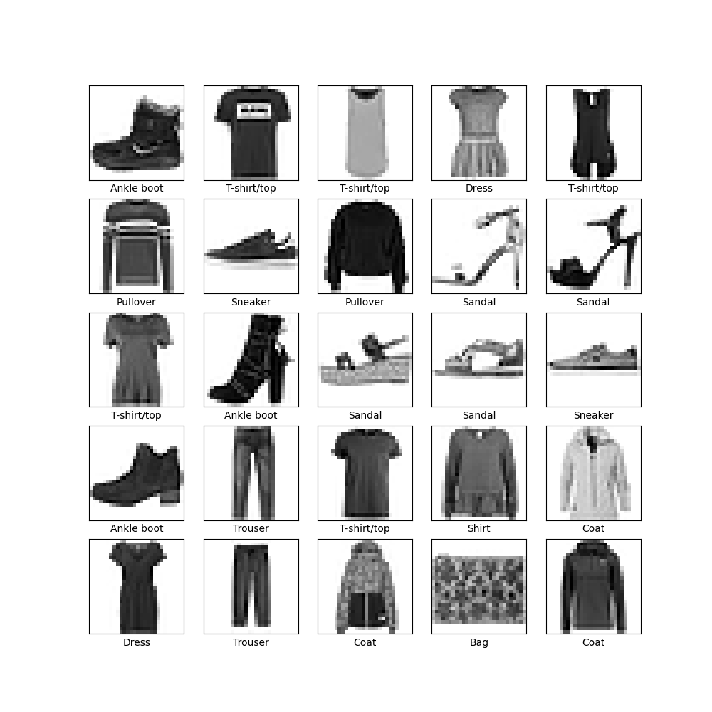
#验证数据的格式是否正确，以及是否已准备好构建和训练网络，显示训练集中的前 25 个图像，并在每个图像下方显示类名称
plt.figure(figsize=(10,10))
for i in range(25):
    plt.subplot(5,5,i+1)
    plt.xticks([])
    plt.yticks([])
    plt.grid(False)
    plt.imshow(train_images[i], cmap=plt.cm.binary)
    plt.xlabel(class_names[train_labels[i]])
plt.show()

7、构建模型

#该网络的第一层 tf.keras.layers.Flatten 将图像格式从二维数组（28 x 28 像素）转换成一维数组（28 x 28 = 784 像素）。将该层视为图像中未堆叠的像素行并将其排列起来。该层没有要学习的参数，它只会重新格式化数据。

展平像素后，网络会包括两个 tf.keras.layers.Dense 层的序列。它们是密集连接或全连接神经层。第一个 Dense 层有 128 个节点（或神经元）。第二个（也是最后一个）层会返回一个长度为 10 的 logits 数组。每个节点都包含一个得分，用来表示当前图像属于 10 个类中的哪一类。
model = keras.Sequential([
    keras.layers.Flatten(input_shape=(28, 28)),
    keras.layers.Dense(128, activation='relu'),
    keras.layers.Dense(10)
])

8、编译模型

#损失函数 - 用于测量模型在训练期间的准确率。您会希望最小化此函数，以便将模型“引导”到正确的方向上。
#优化器 - 决定模型如何根据其看到的数据和自身的损失函数进行更新。
#指标 - 用于监控训练和测试步骤。以下示例使用了准确率，即被正确分类的图像的比率
model.compile(optimizer='adam',
              loss=tf.keras.losses.SparseCategoricalCrossentropy(from_logits=True),
              metrics=['accuracy'])

9、训练模型

训练神经网络模型需要执行以下步骤：

1. 将训练数据馈送给模型。在本例中，训练数据位于 train_images 和 train_labels 数组中。
2. 模型学习将图像和标签关联起来。
3. 要求模型对测试集（在本例中为 test_images 数组）进行预测。
4. 验证预测是否与 test_labels 数组中的标签相匹配。

向模型馈送数据

#调用 model.fit 方法，这样命名是因为该方法会将模型与训练数据进行“拟合”
model.fit(train_images, train_labels, epochs=10)

Epoch 1/10
1875/1875 [==============================] - 3s 2ms/step - loss: 0.4970 - accuracy: 0.8263
Epoch 2/10
1875/1875 [==============================] - 3s 2ms/step - loss: 0.3764 - accuracy: 0.8646
Epoch 3/10
1875/1875 [==============================] - 3s 2ms/step - loss: 0.3386 - accuracy: 0.8768
Epoch 4/10
1875/1875 [==============================] - 3s 2ms/step - loss: 0.3131 - accuracy: 0.8852
Epoch 5/10
1875/1875 [==============================] - 3s 2ms/step - loss: 0.2979 - accuracy: 0.8905
Epoch 6/10
1875/1875 [==============================] - 3s 2ms/step - loss: 0.2817 - accuracy: 0.8946
Epoch 7/10
1875/1875 [==============================] - 3s 2ms/step - loss: 0.2701 - accuracy: 0.8997
Epoch 8/10
1875/1875 [==============================] - 3s 2ms/step - loss: 0.2584 - accuracy: 0.9039
Epoch 9/10
1875/1875 [==============================] - 3s 1ms/step - loss: 0.2494 - accuracy: 0.9071
Epoch 10/10
1875/1875 [==============================] - 3s 2ms/step - loss: 0.2416 - accuracy: 0.9094

评估准确率

#比较模型在测试集上的表现
test_loss, test_acc = model.evaluate(test_images,  test_labels, verbose=2)

print('\nTest accuracy:', test_acc)

Test accuracy: 0.8792999982833862

10、进行预测

#进行预测
probability_model = tf.keras.Sequential([model,
                                         tf.keras.layers.Softmax()])
predictions = probability_model.predict(test_images)
#测试第一个预测结果
print(predictions[0])
#找出置信度最大的标签
print(np.argmax(predictions[0]))
#检查测试标签
print(test_labels[0])

[1.4007558e-08 6.0697776e-09 6.0778667e-08 3.8483901e-08 1.5276806e-08
2.0785581e-03 2.9759491e-07 5.4935408e-03 5.0426343e-07 9.9242699e-01]
9
9

11、绘制图表

def plot_image(i, predictions_array, true_label, img):
  predictions_array, true_label, img = predictions_array, true_label[i], img[i]
  plt.grid(False)
  plt.xticks([])
  plt.yticks([])

  plt.imshow(img, cmap=plt.cm.binary)

  predicted_label = np.argmax(predictions_array)
  if predicted_label == true_label:
    color = 'blue'
  else:
    color = 'red'

  plt.xlabel("{} {:2.0f}% ({})".format(class_names[predicted_label],
                                100*np.max(predictions_array),
                                class_names[true_label]),
                                color=color)

def plot_value_array(i, predictions_array, true_label):
  predictions_array, true_label = predictions_array, true_label[i]
  plt.grid(False)
  plt.xticks(range(10))
  plt.yticks([])
  thisplot = plt.bar(range(10), predictions_array, color="#777777")
  plt.ylim([0, 1])
  predicted_label = np.argmax(predictions_array)

  thisplot[predicted_label].set_color('red')
  thisplot[true_label].set_color('blue')

12、验证预测结果

#对图像进行检测
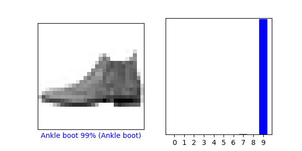
#看看第 0 个图像、预测结果和预测数组。正确的预测标签为蓝色，错误的预测标签为红色。数字表示预测标签的百分比（总计为 100）。
i = 0
plt.figure(figsize=(6,3))
plt.subplot(1,2,1)
plot_image(i, predictions[i], test_labels, test_images)
plt.subplot(1,2,2)
plot_value_array(i, predictions[i],  test_labels)
plt.show()

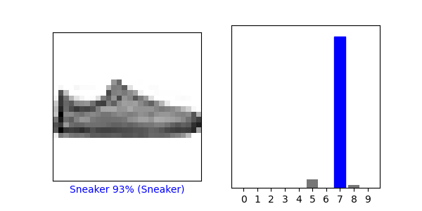
#看第12个图像
i = 12
plt.figure(figsize=(6,3))
plt.subplot(1,2,1)
plot_image(i, predictions[i], test_labels, test_images)
plt.subplot(1,2,2)
plot_value_array(i, predictions[i],  test_labels)
plt.show()

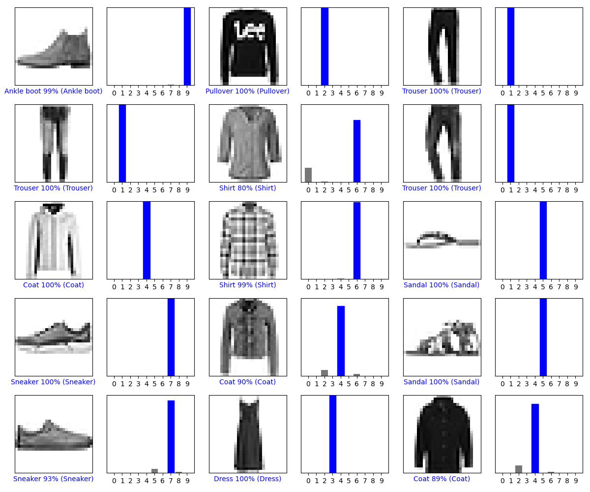
#用模型预测绘制几张图像
# Plot the first X test images, their predicted labels, and the true labels.
# Color correct predictions in blue and incorrect predictions in red.
num_rows = 5
num_cols = 3
num_images = num_rows*num_cols
plt.figure(figsize=(2*2*num_cols, 2*num_rows))
for i in range(num_images):
  plt.subplot(num_rows, 2*num_cols, 2*i+1)
  plot_image(i, predictions[i], test_labels, test_images)
  plt.subplot(num_rows, 2*num_cols, 2*i+2)
  plot_value_array(i, predictions[i], test_labels)
plt.tight_layout()
plt.show()

13、使用训练的模型

使用训练好的模型对单张图片进行预测

#使用训练好的模型对单个图像进行预测
# Grab an image from the test dataset.
img = test_images[1]
print(img.shape)

(28, 28)

#将其添加到列表中
# Add the image to a batch where it's the only member.
img = (np.expand_dims(img,0))

print(img.shape)

(1, 28, 28)

#预测这个图像的正确标签
predictions_single = probability_model.predict(img)

print(predictions_single)

[[1.0675135e-05 2.4023437e-12 9.9772269e-01 1.3299730e-09 1.2968916e-03
  8.7469149e-14 9.6970733e-04 5.4669354e-19 2.4514609e-11 1.8405429e-12]]

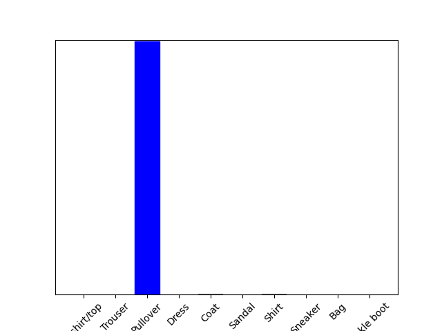
plot_value_array(1, predictions_single[0], test_labels)
_ = plt.xticks(range(10), class_names, rotation=45)

#在批次中获取对我们（唯一）图像的预测
print(np.argmax(predictions_single[0]))

2

14、源代码

# -*- coding = utf-8 -*-
# @Time : 2021/3/16
# @Author : pistachio
# @File : imagesort1.py
# @Software : PyCharm

#导入TensorFlow和tf.keras
import tensorflow as tf
from tensorflow import keras

# Helper libraries
import numpy as np
import matplotlib.pyplot as plt

#从 TensorFlow中导入和加载Fashion MNIST数据
fashion_mnist = keras.datasets.fashion_mnist
(train_images, train_labels), (test_images, test_labels) = fashion_mnist.load_data()

#每个图像都会被映射到一个标签。由于数据集不包括类名称，请将它们存储在下方，供稍后绘制图像时使用
class_names = ['T-shirt/top', 'Trouser', 'Pullover', 'Dress', 'Coat',
               'Sandal', 'Shirt', 'Sneaker', 'Bag', 'Ankle boot']

#这些值缩小至 0 到 1 之间，然后将其馈送到神经网络模型
train_images = train_images / 255.0
test_images = test_images / 255.0

#浏览数据
print(train_images.shape)
print(len(train_labels))
print(train_labels)
print(test_images.shape)
print(len(test_labels))

plt.figure()
plt.imshow(train_images[0])
plt.colorbar()
plt.grid(False)
plt.show()
#为了验证数据的格式是否正确，以及您是否已准备好构建和训练网络，让我们显示训练集中的前 25 个图像，并在每个图像下方显示类名称
plt.figure(figsize=(10, 10))
for i in range(25):
    plt.subplot(5, 5, i+1)
    plt.xticks([])
    plt.yticks([])
    plt.grid(False)
    plt.imshow(train_images[i], cmap=plt.cm.binary)
    plt.xlabel(class_names[train_labels[i]])
plt.show()

#训练模型
model = keras.Sequential([
    keras.layers.Flatten(input_shape=(28, 28)),
    keras.layers.Dense(128, activation='relu'),
    keras.layers.Dense(10)
])

model.compile(optimizer='adam',
              loss=tf.keras.losses.SparseCategoricalCrossentropy(from_logits=True),
              metrics=['accuracy'])

model.fit(train_images, train_labels, epochs=10)

test_loss, test_acc = model.evaluate(test_images,  test_labels, verbose=2)

print('\nTest accuracy:', test_acc)

#进行预测
probability_model = tf.keras.Sequential([model,
                                         tf.keras.layers.Softmax()])
predictions = probability_model.predict(test_images)
#测试第一个预测结果
print(predictions[0])
#找出置信度最大的标签
print(np.argmax(predictions[0]))
#检查测试标签
print(test_labels[0])

#将其绘制成图表，看看模型对于全部 10 个类的预测
def plot_image(i, predictions_array, true_label, img):
  predictions_array, true_label, img = predictions_array, true_label[i], img[i]
  plt.grid(False)
  plt.xticks([])
  plt.yticks([])

  plt.imshow(img, cmap=plt.cm.binary)

  predicted_label = np.argmax(predictions_array)
  if predicted_label == true_label:
    color = 'blue'
  else:
    color = 'red'

  plt.xlabel("{} {:2.0f}% ({})".format(class_names[predicted_label],
                                100*np.max(predictions_array),
                                class_names[true_label]),
                                color=color)

def plot_value_array(i, predictions_array, true_label):
  predictions_array, true_label = predictions_array, true_label[i]
  plt.grid(False)
  plt.xticks(range(10))
  plt.yticks([])
  thisplot = plt.bar(range(10), predictions_array, color="#777777")
  plt.ylim([0, 1])
  predicted_label = np.argmax(predictions_array)

  thisplot[predicted_label].set_color('red')
  thisplot[true_label].set_color('blue')

#对图像进行检测
#看看第 0 个图像、预测结果和预测数组。正确的预测标签为蓝色，错误的预测标签为红色。数字表示预测标签的百分比（总计为 100）。
i = 0
plt.figure(figsize=(6,3))
plt.subplot(1,2,1)
plot_image(i, predictions[i], test_labels, test_images)
plt.subplot(1,2,2)
plot_value_array(i, predictions[i],  test_labels)
plt.show()
#看第12个图像
i = 12
plt.figure(figsize=(6,3))
plt.subplot(1,2,1)
plot_image(i, predictions[i], test_labels, test_images)
plt.subplot(1,2,2)
plot_value_array(i, predictions[i],  test_labels)
plt.show()
#用模型预测绘制几张图像
# Plot the first X test images, their predicted labels, and the true labels.
# Color correct predictions in blue and incorrect predictions in red.
num_rows = 5
num_cols = 3
num_images = num_rows*num_cols
plt.figure(figsize=(2*2*num_cols, 2*num_rows))
for i in range(num_images):
  plt.subplot(num_rows, 2*num_cols, 2*i+1)
  plot_image(i, predictions[i], test_labels, test_images)
  plt.subplot(num_rows, 2*num_cols, 2*i+2)
  plot_value_array(i, predictions[i], test_labels)
plt.tight_layout()
plt.show()

#使用训练好的模型对单个图像进行预测
# Grab an image from the test dataset.
img = test_images[1]
print(img.shape)

#将其添加到列表中
# Add the image to a batch where it's the only member.
img = (np.expand_dims(img,0))
print(img.shape)

#预测这个图像的正确标签
predictions_single = probability_model.predict(img)

print(predictions_single)

plot_value_array(1, predictions_single[0], test_labels)
_ = plt.xticks(range(10), class_names, rotation=45)
plt.show()
print(np.argmax(predictions_single[0]))