在树莓派上实现numpy的LSTM长短期记忆神经网络做图像分类，加载pytorch的模型参数，推理mnist手写数字识别

这几天又在玩树莓派，先是搞了个物联网，又在尝试在树莓派上搞一些简单的神经网络，这次搞得是LSTM识别mnist手写数字识别

训练代码在电脑上，cpu就能训练，很快的：

import torch
import torch.nn as nn
import torchvision
import numpy as np
import os
from PIL import Image

# 定义LSTM模型
class LSTMModel(nn.Module):
    def __init__(self, input_size, hidden_size, num_layers, num_classes):
        super(LSTMModel, self).__init__()
        self.hidden_size = hidden_size
        self.num_layers = num_layers
        self.lstm = nn.LSTM(input_size, hidden_size, num_layers, batch_first=True)
        self.fc = nn.Linear(hidden_size, num_classes)

    def forward(self, x):
        h0 = torch.zeros(self.num_layers, x.size(0), self.hidden_size).to(x.device)
        c0 = torch.zeros(self.num_layers, x.size(0), self.hidden_size).to(x.device)

        out, (h_n,c_n) = self.lstm(x, (h0, c0))
        out = self.fc(out[:, -1, :])
        return out

# 设置超参数
input_size = 28
sequence_length = 28
hidden_size = 128
num_layers = 2
num_classes = 10
batch_size = 100
num_epochs = 1
learning_rate = 0.001

# 加载MNIST数据集
train_dataset = torchvision.datasets.MNIST(root='./data', train=True, transform=torchvision.transforms.ToTensor(), download=True)
test_dataset = torchvision.datasets.MNIST(root='./data', train=False, transform=torchvision.transforms.ToTensor())

# 创建数据加载器
train_loader = torch.utils.data.DataLoader(dataset=train_dataset, batch_size=batch_size, shuffle=True)
test_loader = torch.utils.data.DataLoader(dataset=test_dataset, batch_size=batch_size, shuffle=False)

# 创建LSTM模型
model = LSTMModel(input_size, hidden_size, num_layers, num_classes)

# 定义损失函数和优化器
criterion = nn.CrossEntropyLoss()
optimizer = torch.optim.Adam(model.parameters(), lr=learning_rate)

# 训练模型
total_step = len(train_loader)
for epoch in range(num_epochs):
    for i, (images, labels) in enumerate(train_loader):
        images = images.reshape(-1, sequence_length, input_size)
        outputs = model(images)
        loss = criterion(outputs, labels)

        predictions = torch.argmax(outputs,dim=1)
        # acc = torch.eq(predictions,labels).sum().item()
        # print(acc)
        optimizer.zero_grad()
        loss.backward()
        optimizer.step()

        if (i + 1) % 100 == 0:
            print('Epoch [{}/{}], Step [{}/{}], Loss: {:.4f}'.format(epoch + 1, num_epochs, i + 1, total_step, loss.item()))

# 保存模型
torch.save(model.state_dict(), 'model.pth')

# 加载模型
model.load_state_dict(torch.load('model.pth'))
with torch.no_grad():
    for i, (images, labels) in enumerate(test_loader):
        images = images.reshape(-1, sequence_length, input_size)
        outputs = model(images)
        predictions = torch.argmax(outputs,dim=1)
        acc = torch.eq(predictions,labels).sum().item()
        print(acc)

# folder_path = './mnist_pi'  # 替换为图片所在的文件夹路径
# def infer_images_in_folder(folder_path):
#     with torch.no_grad():
#         for file_name in os.listdir(folder_path):
#             file_path = os.path.join(folder_path, file_name)
#             if os.path.isfile(file_path) and file_name.endswith(('.jpg', '.jpeg', '.png')):
#                 image = Image.open(file_path)
#                 label = file_name.split(".")[0].split("_")[1]
#                 image = np.array(image)/255.0
#                 image = np.expand_dims(image,axis=0)
#                 image= torch.tensor(image).to(torch.float32)
#                 logits = model(image)
#                 predicted_class = torch.argmax(logits)
#                 print("file_path:",file_path,"img size:",image.shape,"label:",label,'Predicted class:', predicted_class)
#             break

# infer_images_in_folder(folder_path)

# 保存模型参数为numpy的数组格式
model_params = {}
# print(list(model.parameters()))
for name, param in model.named_parameters():
    model_params[name] = param.detach().numpy()
    print(name,param.shape)

np.savez('model.npz', **model_params)

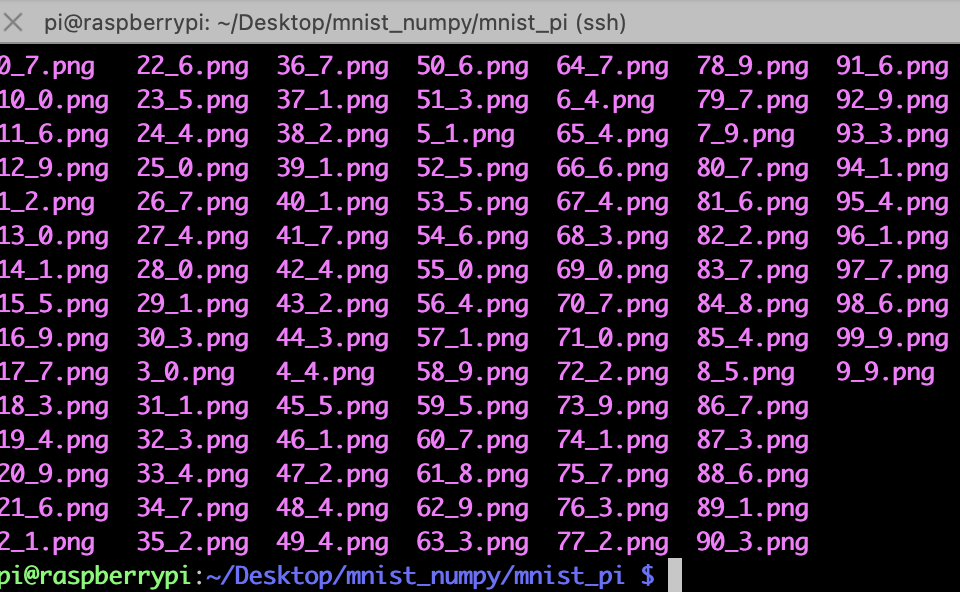
然后需要自己在dataset里导出一些图片：我保存在了mnist_pi文件夹下,“_”后面的是标签，主要是在pc端导出保存到树莓派下

树莓派推理端的代码，需要numpy手动重新搭建网络，并且需要手动实现双层的LSTM神经网络，然后加载那些保存的矩阵参数，做矩阵乘法和加法

import numpy as np
import os
from PIL import Image

# 加载模型参数
model_data = np.load('model.npz')

'''
weight_ih_l[k] : the learnable input-hidden weights of the :math:`\text{k}^{th}` layer
    `(W_ii|W_if|W_ig|W_io)`, of shape `(4*hidden_size, input_size)` for `k = 0`.
    Otherwise, the shape is `(4*hidden_size, num_directions * hidden_size)`. If
    ``proj_size > 0`` was specified, the shape will be
    `(4*hidden_size, num_directions * proj_size)` for `k > 0`
weight_hh_l[k] : the learnable hidden-hidden weights of the :math:`\text{k}^{th}` layer
    `(W_hi|W_hf|W_hg|W_ho)`, of shape `(4*hidden_size, hidden_size)`. If ``proj_size > 0``
    was specified, the shape will be `(4*hidden_size, proj_size)`.
bias_ih_l[k] : the learnable input-hidden bias of the :math:`\text{k}^{th}` layer
    `(b_ii|b_if|b_ig|b_io)`, of shape `(4*hidden_size)`
bias_hh_l[k] : the learnable hidden-hidden bias of the :math:`\text{k}^{th}` layer
    `(b_hi|b_hf|b_hg|b_ho)`, of shape `(4*hidden_size)`
'''

# 提取模型参数
lstm_weight_ih_l0 = model_data['lstm.weight_ih_l0']
lstm_weight_hh_l0 = model_data['lstm.weight_hh_l0']
lstm_bias_ih_l0 = model_data['lstm.bias_ih_l0']
lstm_bias_hh_l0 = model_data['lstm.bias_hh_l0']
lstm_weight_ih_l1 = model_data['lstm.weight_ih_l1']
lstm_weight_hh_l1 = model_data['lstm.weight_hh_l1']
lstm_bias_ih_l1 = model_data['lstm.bias_ih_l1']
lstm_bias_hh_l1 = model_data['lstm.bias_hh_l1']
fc_weight = model_data['fc.weight']
fc_bias = model_data['fc.bias']

# print(lstm_weight_ih_l0.shape,lstm_weight_hh_l0.shape)
# print(lstm_bias_ih_l0.shape,lstm_bias_hh_l0.shape)
# 定义LSTM模型
def lstm_model(inputs):
    '''
        踩到两个坑，一个是矩阵形状都是这种(4*hidden_size, hidden_size)合并的，需要拆分。
        另一个坑是，两层的lstm层需要每个时间步的输出都输入到下一层，而不是最后一个时间步的数据给下一层
    '''

    batch_size, sequence_length, input_size = inputs.shape
    hidden_size = lstm_weight_hh_l0.shape[1]
    num_classes = fc_weight.shape[0]

    h0 = np.zeros((batch_size, hidden_size))
    c0 = np.zeros((batch_size, hidden_size))

    # 第一层LSTM
    h_l0, c_l0 = np.zeros_like(h0), np.zeros_like(c0)
    out_0 = []
    for t in range(sequence_length):
        x = inputs[:, t, :]
        '''
        i_t = \sigma(W_{ii} x_t + b_{ii} + W_{hi} h_{t-1} + b_{hi}) \\
        f_t = \sigma(W_{if} x_t + b_{if} + W_{hf} h_{t-1} + b_{hf}) \\
        g_t = \tanh(W_{ig} x_t + b_{ig} + W_{hg} h_{t-1} + b_{hg}) \\
        o_t = \sigma(W_{io} x_t + b_{io} + W_{ho} h_{t-1} + b_{ho}) \\
        c_t = f_t \odot c_{t-1} + i_t \odot g_t \\
        h_t = o_t \odot \tanh(c_t) \\
        '''
        # 输入门
        i_t = sigmoid(np.dot(x, lstm_weight_ih_l0[:128].T) + np.dot(h_l0, lstm_weight_hh_l0[:128].T) + lstm_bias_ih_l0[:128] + lstm_bias_hh_l0[:128])
        # 遗忘门
        f_t = sigmoid(np.dot(x, lstm_weight_ih_l0[128:256].T) + np.dot(h_l0, lstm_weight_hh_l0[128:256].T) + lstm_bias_ih_l0[128:256] + lstm_bias_hh_l0[128:256])
        # 候选向量
        g_t = np.tanh(np.dot(x, lstm_weight_ih_l0[256:256+128].T) + np.dot(h_l0, lstm_weight_hh_l0[256:256+128].T) + lstm_bias_ih_l0[256:256+128] + lstm_bias_hh_l0[256:256+128])
        # 输出门
        o_t = sigmoid(np.dot(x, lstm_weight_ih_l0[256+128:512].T) + np.dot(h_l0, lstm_weight_hh_l0[256+128:512].T) + lstm_bias_ih_l0[256+128:512] + lstm_bias_hh_l0[256+128:512])
        # 细胞状态
        c_l0 = f_t * c_l0 + i_t * g_t
        # 隐藏状态
        h_l0 = o_t * np.tanh(c_l0)
        out_0.append(h_l0)

    # 第二层LSTM
    h_l1, c_l1 = np.zeros_like(h0), np.zeros_like(c0)
    out_1 = []
    for t in range(sequence_length):
        x = out_0[t]
        # 输入门
        i_t = sigmoid(np.dot(x, lstm_weight_ih_l1[:128].T) + np.dot(h_l1, lstm_weight_hh_l1[:128].T) + lstm_bias_ih_l1[:128] + lstm_bias_hh_l1[:128])
        # 遗忘门
        f_t = sigmoid(np.dot(x, lstm_weight_ih_l1[128:256].T) + np.dot(h_l1, lstm_weight_hh_l1[128:256].T) + lstm_bias_ih_l1[128:256] + lstm_bias_hh_l1[128:256])
        # 候选向量
        g_t = np.tanh(np.dot(x, lstm_weight_ih_l1[256:256+128].T) + np.dot(h_l1, lstm_weight_hh_l1[256:256+128].T) + lstm_bias_ih_l1[256:256+128] + lstm_bias_hh_l1[256:256+128])
        # 输出门
        o_t = sigmoid(np.dot(x, lstm_weight_ih_l1[256+128:512].T) + np.dot(h_l1, lstm_weight_hh_l1[256+128:512].T) + lstm_bias_ih_l1[256+128:512] + lstm_bias_hh_l1[256+128:512])
        # 细胞状态
        c_l1 = f_t * c_l1 + i_t * g_t
        # 隐藏状态
        h_l1 = o_t * np.tanh(c_l1)
        out_1.append(h_l1)

    # 全连接层
    fc_output = np.dot(h_l1, fc_weight.T) + fc_bias
    predictions = np.argmax(fc_output, axis=1)
    return predictions

# Sigmoid激活函数
def sigmoid(x):
    return 1 / (1 + np.exp(-x))

folder_path = './mnist_pi'  # 替换为图片所在的文件夹路径
def infer_images_in_folder(folder_path):
    for file_name in os.listdir(folder_path):
        file_path = os.path.join(folder_path, file_name)
        if os.path.isfile(file_path) and file_name.endswith(('.jpg', '.jpeg', '.png')):
            image = Image.open(file_path)
            label = file_name.split(".")[0].split("_")[1]
            image = np.array(image)/255.0
            image = np.expand_dims(image,axis=0)
            predicted_class = lstm_model(image)
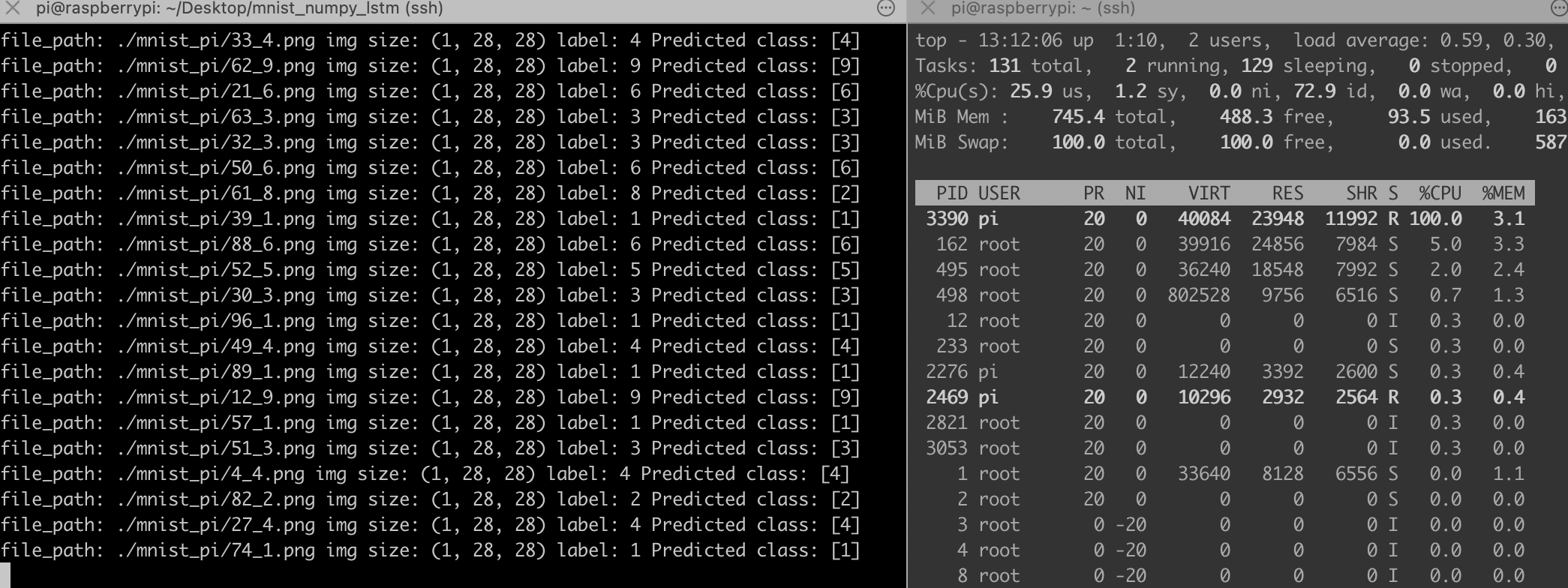
            print("file_path:",file_path,"img size:",image.shape,"label:",label,'Predicted class:', predicted_class)

infer_images_in_folder(folder_path)

这代码完全就是numpy推理，不需要安装pytorch，树莓派也装不动pytorch，太重了，下面是推理结果，比之前的MLP网络慢很多，主要是手动实现的LSTM网络全靠循环实现。