Keras 自适应Learning Rate (LearningRateScheduler)

When training deep neural networks, it is often useful to reduce learning rate as the training progresses. This can be done by using pre-defined learning rate schedules or adaptive learning rate methods. In this article, I train a convolutional neural network on CIFAR-10 using differing learning rate schedules and adaptive learning rate methods to compare their model performances.

Learning Rate Schedules

Learning rate schedules seek to adjust the learning rate during training by reducing the learning rate according to a pre-defined schedule. Common learning rate schedules include time-based decay, step decay and exponential decay. For illustrative purpose, I construct a convolutional neural network trained on CIFAR-10, using stochastic gradient descent (SGD) optimization algorithm with different learning rate schedules to compare the performances.

Constant Learning Rate

Constant learning rate is the default learning rate schedule in SGD optimizer in Keras. Momentum and decay rate are both set to zero by default. It is tricky to choose the right learning rate. By experimenting with range of learning rates in our example, lr=0.1 shows a relative good performance to start with. This can serve as a baseline for us to experiment with different learning rate strategies.

keras.optimizers.SGD(lr=0.1, momentum=0.0, decay=0.0, nesterov=False)

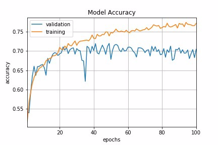
Fig 1 : Constant Learning Rate

Time-Based Decay

The mathematical form of time-based decay is lr = lr0/(1+kt) where lr, k are hyperparameters and t is the iteration number. Looking into the source code of Keras, the SGD optimizer takes decay and lr arguments and update the learning rate by a decreasing factor in each epoch.

lr *= (1. / (1. + self.decay * self.iterations))

Momentum is another argument in SGD optimizer which we could tweak to obtain faster convergence. Unlike classical SGD, momentum method helps the parameter vector to build up velocity in any direction with constant gradient descent so as to prevent oscillations. A typical choice of momentum is between 0.5 to 0.9.

SGD optimizer also has an argument called nesterov which is set to false by default. Nesterov momentum is a different version of the momentum method which has stronger theoretical converge guarantees for convex functions. In practice, it works slightly better than standard momentum.

In Keras, we can implement time-based decay by setting the initial learning rate, decay rate and momentum in the SGD optimizer.

learning_rate = 0.1

decay_rate = learning_rate / epochs

momentum = 0.8

sgd = SGD(lr=learning_rate, momentum=momentum, decay=decay_rate, nesterov=False)

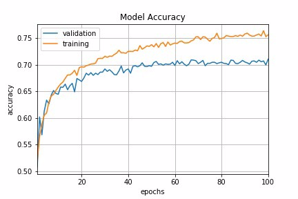
Fig 2 : Time-based Decay Schedule

Step Decay

Step decay schedule drops the learning rate by a factor every few epochs. The mathematical form of step decay is :

lr = lr0 * drop^floor(epoch / epochs_drop)

A typical way is to to drop the learning rate by half every 10 epochs. To implement this in Keras, we can define a step decay function and use LearningRateScheduler callback to take the step decay function as argument and return the updated learning rates for use in SGD optimizer.

def step_decay(epoch):

   initial_lrate = 0.1

   drop = 0.5

   epochs_drop = 10.0

   lrate = initial_lrate * math.pow(drop,

           math.floor((1+epoch)/epochs_drop))

   return lrate

lrate = LearningRateScheduler(step_decay)

As a digression, a callback is a set of functions to be applied at given stages of the training procedure. We can use callbacks to get a view on internal states and statistics of the model during training. In our example, we create a custom callback by extending the base class keras.callbacks.Callback to record loss history and learning rate during the training procedure.

class LossHistory(keras.callbacks.Callback):

    def on_train_begin(self, logs={}):

       self.losses = []

       self.lr = []

    def on_epoch_end(self, batch, logs={}):

       self.losses.append(logs.get(‘loss’))

       self.lr.append(step_decay(len(self.losses)))

Putting everything together, we can pass a callback list consisting of LearningRateScheduler callback and our custom callback to fit the model. We can then visualize the learning rate schedule and the loss history by accessing loss_history.lr and loss_history.losses.

loss_history = LossHistory()

lrate = LearningRateScheduler(step_decay)

callbacks_list = [loss_history, lrate]

history = model.fit(X_train, y_train,

   validation_data=(X_test, y_test),

   epochs=epochs,

   batch_size=batch_size,

   callbacks=callbacks_list,

   verbose=2)

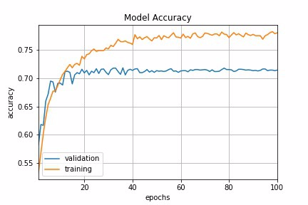
Fig 3a : Step Decay Schedule

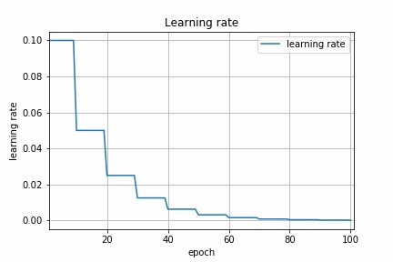
Fig 3b : Step Decay Schedule

Exponential Decay

Another common schedule is exponential decay. It has the mathematical form lr = lr0 * e^(−kt), where lr, k are hyperparameters and t is the iteration number. Similarly, we can implement this by defining exponential decay function and pass it to LearningRateScheduler. In fact, any custom decay schedule can be implemented in Keras using this approach. The only difference is to define a different custom decay function.

def exp_decay(epoch):

   initial_lrate = 0.1

   k = 0.1

   lrate = initial_lrate * exp(-k*t)

   return lrate

lrate = LearningRateScheduler(exp_decay)

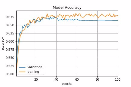
Fig 4a : Exponential Decay Schedule

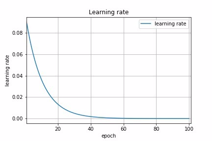
Fig 4b : Exponential Decay Schedule

Let us now compare the model accuracy using different learning rate schedules in our example.

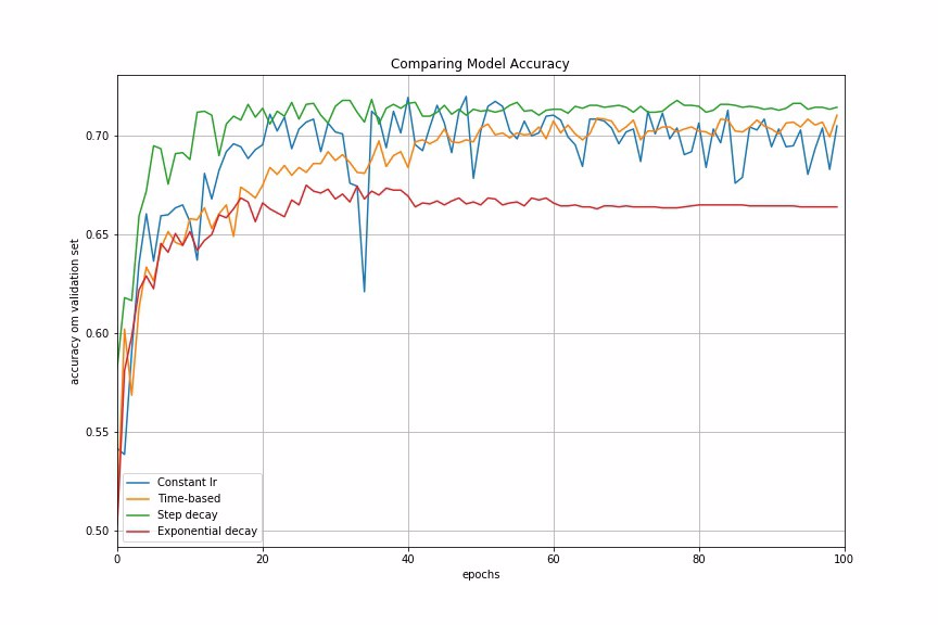
Fig 5 : Comparing Performances of Different Learning Rate Schedules

Adaptive Learning Rate Methods

The challenge of using learning rate schedules is that their hyperparameters have to be defined in advance and they depend heavily on the type of model and problem. Another problem is that the same learning rate is applied to all parameter updates. If we have sparse data, we may want to update the parameters in different extent instead.

Adaptive gradient descent algorithms such as Adagrad, Adadelta, RMSprop, Adam, provide an alternative to classical SGD. These per-parameter learning rate methods provide heuristic approach without requiring expensive work in tuning hyperparameters for the learning rate schedule manually.

In brief, Adagrad performs larger updates for more sparse parameters and smaller updates for less sparse parameter. It has good performance with sparse data and training large-scale neural network. However, its monotonic learning rate usually proves too aggressive and stops learning too early when training deep neural networks. Adadelta is an extension of Adagrad that seeks to reduce its aggressive, monotonically decreasing learning rate. RMSprop adjusts the Adagrad method in a very simple way in an attempt to reduce its aggressive, monotonically decreasing learning rate. Adam is an update to the RMSProp optimizer which is like RMSprop with momentum.

In Keras, we can implement these adaptive learning algorithms easily using corresponding optimizers. It is usually recommended to leave the hyperparameters of these optimizers at their default values (except lrsometimes).

keras.optimizers.Adagrad(lr=0.01, epsilon=1e-08, decay=0.0)

keras.optimizers.Adadelta(lr=1.0, rho=0.95, epsilon=1e-08, decay=0.0)

keras.optimizers.RMSprop(lr=0.001, rho=0.9, epsilon=1e-08, decay=0.0)

keras.optimizers.Adam(lr=0.001, beta_1=0.9, beta_2=0.999, epsilon=1e-08, decay=0.0)

Let us now look at the model performances using different adaptive learning rate methods. In our example, Adadelta gives the best model accuracy among other adaptive learning rate methods.

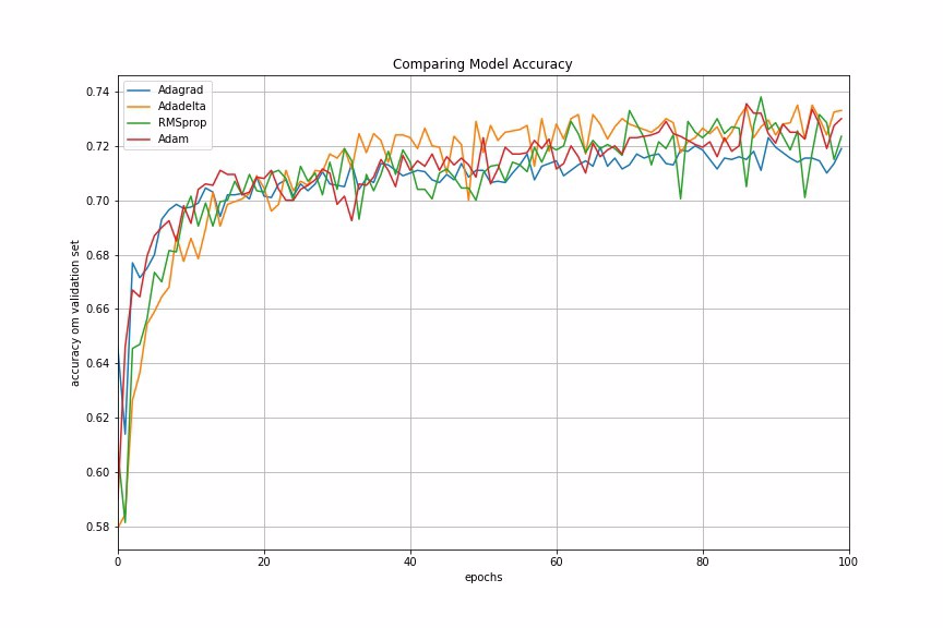
Fig 6 : Comparing Performances of Different Adaptive Learning Algorithms

Finally, we compare the performances of all the learning rate schedules and adaptive learning rate methods we have discussed.

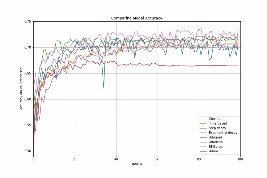
Fig 7: Comparing Performances of Different Learning Rate Schedules and Adaptive Learning Algorithms

Conclusion

In many examples I have worked on, adaptive learning rate methods demonstrate better performance than learning rate schedules, and they require much less effort in hyperparamater settings. We can also use LearningRateScheduler in Keras to create custom learning rate schedules which is specific to our data problem.

For further reading, Yoshua Bengio’s paper provides very good practical recommendations for tuning learning rate for deep learning, such as how to set initial learning rate, mini-batch size, number of epochs and use of early stopping and momentum.

Source code

References:

来源： https://towardsdatascience.com/learning-rate-schedules-and-adaptive-learning-rate-methods-for-deep-learning-2c8f433990d1

==============================================================

keras.callbacks.LearningRateScheduler(schedule)
该回调函数是用于动态设置学习率
参数：
● schedule：函数，该函数以epoch号为参数（从0算起的整数），返回一个新学习率（浮点数）

示例：

from keras.callbacks import LearningRateScheduler

lr_base = 0.001

epochs = 250

lr_power = 0.9

def lr_scheduler(epoch, mode='power_decay'):

    '''if lr_dict.has_key(epoch):

        lr = lr_dict[epoch]

        print 'lr: %f' % lr'''

    if mode is 'power_decay':

        # original lr scheduler

        lr = lr_base * ((1 - float(epoch) / epochs) ** lr_power)

    if mode is 'exp_decay':

        # exponential decay

        lr = (float(lr_base) ** float(lr_power)) ** float(epoch + 1)

    # adam default lr

    if mode is 'adam':

        lr = 0.001

    if mode is 'progressive_drops':

        # drops as progression proceeds, good for sgd

        if epoch > 0.9 * epochs:

            lr = 0.0001

        elif epoch > 0.75 * epochs:

            lr = 0.001

        elif epoch > 0.5 * epochs:

            lr = 0.01

        else:

            lr = 0.1

    print('lr: %f' % lr)

    return lr

# 学习率调度器

scheduler = LearningRateScheduler(lr_scheduler)

来源： https://blog.csdn.net/hanshuobest/article/details/78882334