Tree - AdaBoost with sklearn source code

In the previous post we addressed some issue of decision tree, including instability, lack of smoothness, sensitivity to data, and etc.

One solution is Boosting Method. In simple words Boosting combines multiple weak learners to get a powerful prediction, where the weak learner are usually shallow tree.

Before we go to the popularly used boosting algorithm like GBM(GBRT) and xgBoost, let's start with one of the earliest Boosting Method - AdaBoost.

AdaBoost Evolution

Early AdaBoost focus on binary classification only. And then it extend to regression problem and multi-class classification. Let's go through them one by one.

Discrete AdaBoost (Freund & Schapire 1996)

A concise description of Discrete AdaBoost is that at each step a base binary classifier ($f_m(x) \in \{-1,1 \}$) is trained against a weighted training sample. The weight of misclassified sample will increase, and then another classifier will be trained with updated weight. The final result will be a weighted sum of all base classifiers.

assign equal weight to all sample $w_i = 1/N$

Repeat below m times

A. Fit classifier $f_m(x) \in \{-1,1\}$, by minimizing a weighted loss function

B. Compute weighted misclassification rate $e_m = E_w[I(y\ne f_m(x))] = \sum_i{w_i \cdot I(y\ne f_m(x)) }$

C. Compute classifier weight $c_m = log((1-e_m)/e_m)$

D. Update sample weight $w_i = w_i * exp(c_m \cdot I(y\ne f_m(x))$

E. Normalize weight so that $\sum_i{w_i} = 1$

Output the classifier $sign[\sum_{i=1}^M c_m f_m(x)]$

A few intuitive finding of the above algorithm:

The bigger the error for the base learner, the lower weight it will have.
If the weighted miscalssification rate is higher than 50%, which is worse then random guess, then this base learner will get negative weight.
The smaller the error for the base learner, the weight of misclassified sample will increase more.

I guess most of people may be curious why the weight is updated in above way, and why a sequence of weak learner can be better than a single classifier. We will get to this magic later.

Real AdaBoost (Schapire & Singer 1998)

Above discrete AdaBoost is limited to binary classification. A more generalized AdaBoost called Real AdaBoost is developed later, where probability ($P_m(x) \in [0,1])$) is trained at each step, like logistics regression.

With some modification on discrete algo, we get below:

Assign equal weight to all sample $w_i = 1/N$

Repeat below m times

A. Fit classier $p_m(x) \in [-1,1]$, by minimizing a weighted loss function

B. Compute $f_m(x) = \frac{1}{2}log(p_m(x)/(1-p_m(x)) )$

C. Update weight: $w_i = w_i * exp(-y_if_m(x_i) )$

D. Normalize weight so that $\sum_i{w_i} = 1$

Output the classifier $sign[\sum_{i=1}^M f_m(x)]$

Discrete Multi-class AdaBoost (J. Zhu, et al 2009)

Later the AdaBoost algorithm is further extended to multi-class classification. This is also the algorithm currently used in sklearn. For a k-class classification problem, the algo is below

assign equal weight to all sample $w_i = 1/N$

Repeat below m times

A. Fit classifier $f_m(x)$ by minimizing a weighted loss function

B. Compute weighted misclassification rate $e_m = E_w[I(y\ne f_m(x))] = \sum_i{w_i \cdot I(y\ne f_m(x)) }$

C. Compute classifier weight $c_m = log((1-e_m)/e_m) + log(K-1)$

D. Update sample weight $w_i = w_i * exp(c_m \cdot I(y\ne f_m(x))$

E. Normalize weight so that $\sum_i{w_i} = 1$

Output the classifier $argmax{\sum_{i=1}^M c_m \cdot I(f_m(x)=k)}$

Here we can see when k=2, the multi-class AdaBoost will be the same as original AdaBoost. The biggest difference lies in weight calculation. For original AdaBoost, there is a stopping threshold that each weak classifier weight must be greater >0, meaning misclassification rate should be smaller than 50% (purely random).

However for multi-class, we allow misclassification rate to be bigger than 50%, in other words we tends to overweight misclassified sample more than 2-class AdaBoost.

Why AdaBoost work? (Friedman et al. 2000)

Noe let's try to solve your confusion:

Why train weak learner additively?
Why the sample weight is updated in this way?
Why the final ensemble is done in this way?

Friedman reveals the mystery in 2000, where he shows AdaBoost is a forward stage-wise additive model, by minimizing exponential loss . 2 main assumptions here:

$F(x) = \sum_{m=1}^Mc_m f_m(x)$ AdaBoost can be decomposed into a weighted additive function, where new basis function is sequentially added to the expansion without adjusting the existing term.
$J(F) = E(e^{(-yF(x))})$ AdaBoost approximate the exponential loss iteratively.

Algorithm reproduction

Now let's work the magic and reproduce the discrete AdaBoost algorithm.

Based on current $F(x)$ estimator for $y \in \{-1,1\}$, we additively compute $f(x) \in \{-1,1\}$ by minimizing $J(F(x) + cf(x))$

\[\begin{align}
J(F(x) +cf(x)) &= E(exp{(-y(F(x) + cf(x)) }) \\
&= \sum_{i=1}^N{w_i *exp{-ycf(x)}}\\
&= \sum_{y=f(x)} w_i \cdot e^{-c} + \sum_{y \neq f(x)} w_i \cdot e^{c} \\
&= \sum_{i=1}^{N} w_i \cdot e^{-c} + \sum_{y \neq f(x)} w_i \cdot (e^{c} - e^{-c} ) \\
& = e^{-c} + \sum_{y \neq f(x)} w_i \cdot (e^{c} - e^{-c} )\\
& = e^{-c} + (e^{c} - e^{-c} ) \sum w_i \cdot I(y \neq f(x))
\end{align}
\]

Therefore

\[ \text{argmin } {J(F(x) + cf(x)) }= \text{argmin }\sum w_i \cdot I(y \neq f(x))
\]

So we minimize weighted misclassification rate to get base learner at each iteration, exactly the same as step 2(A) in AdaBoost, where sample weight is the current exponential error.

After solving misclassification rate $e_m$, we further solve base learner coefficient c

\[\begin{align}
& \text{min }{ e^{-c} + (e^{c} - e^{-c}) \cdot e_m }\\
& \text{where c} =\frac{1}{2} \log{\frac{1-e_m}{e_m} = \frac{1}{2} c_m }
\end{align}
\]

Constant 0.5 is same for all base learner. Ignoring it, we will get the same coefficient as step 2(C) in AdaBoost.

Last let's see how the weighted is update

\[\begin{align}
w'_i & = e^{ -y(F(x)+cf(x) )} \\
& = w_i \cdot \exp{(2I(y \neq f(x)-1)\cdot c} \\
& = w_i \cdot \exp{(I(y \neq f(x)) \cdot c_m)} * constant
\end{align}
\]

Since the weight is always normalized, ignoring constant we will get the same weight updating formula as step 2(D) in AdaBoost.

Boom! So far we already proved that AdaBoost is approximating an exponential error with a forward additive model. Next let's dig even deeper, what exactly is exponential loss solving?

Algorithm Insight

Let's recall the loss function for classification problem that we discussed in previous tree model. We have misclassification rate, Gini Index and cross-entropy (negative log-likelihood ). Then what is exponential loss solving?

Idea 1. Exponential loss can be approximated via AdaBoost

Actually when AdaBoost is first invented, author didn't think in terms of exponential loss, which is proved by Freud 5 years later.

Therefore first usage of exponential loss is that it can be approximated by additive model. By iteratively training weak classifier and re-weighting sample with misclassification rate, we can approximate exponential loss.

Idea 2. Exponential loss solves for Logit function

Let's use the binary classification problem as an example to solve the loss function. Here $y \in \{-1,1\}$ and $sign(f(x))$ is the binary prediction.

\[\begin{align}
E(\exp{-yf(x)} | X ) &= e^{-f(x)}E(I(y=1)|x) + e^{f(x)} E(y=-1|x)\\
& = e^{-f(x)}P(y=1|x) + e^{f(x)}P(y=-1|x)\\
\frac{\partial E(\exp{-yf(x)} | X )}{\partial f(x)} & = - e^{-f(x)}P(y=1|x) + e^{f(x)}(1-P) \\
f(x) &= \frac{1}{2}\log{\frac{p}{1-p}}
\end{align}
\]

Does $f(x)$ looks familiar to you? Yes it is the half Logit function (log-odds)! In logistics regression we use above formula to map $x \in R \to y \in \{0,1\}$

Let's have a brief review of logistic regression.

when $y \in \{0,1\}$

\[\begin{align}
P = P(y= 1|x) &= \frac{1}{1+e^{-f(x)}} \\
\text{ And }f(x) & = \log{\frac{p}{1-p}}
\end{align}
\]

when $y \in \{-1,1\}$, modification is needed

\[\begin{align}
P = P(y=1|x) &= \frac{1}{1+e^{-yf(x)}}
\end{align}
\]

The cross-entropy (negative log-likelihood) is defined below.

\[\begin{align}
L(Y,p(x)) &= - E(I(y=1)\log{p(x)} +I(y=-1)\log{1-p(x)} )\\
&= E(\log{(1+ \exp{-yf(x)} )})
\end{align}
\]

Boom! Logistics Regression actually is optimizing a similar loss function, compared to exponential Loss.

Idea 3. Exponentional loss is a differentiable representation of misclassificaton error

In both exponential loss and negative log-likelihood, we can see loss is monotone decreasing of $yf(x)$ (margin), which is similar to residual $y-f(x)$ in regression problem. Decision boundary for $yf(x)$ is 0, where $yf(x)>0$ is correctly classified.

Compared to misclassifcation error $I(yf(x)<0)$, the advantage of $yf(x)$ is that even if misclassification rate is 0, the model training will keep pushing the sample to be more distinguishly separated, meaning f(x) may have bigger absolute value.

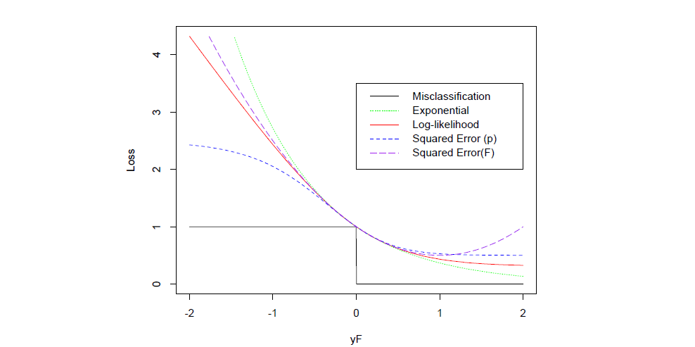
Above is a comparison between different loss function (scaled to cross(0,1)). A few take away here

Compare with Squared Error (F), exponential loss is monotonically decreasing with $yf(x)$, it doesn't penalize sample that are too correctly classified.
Both exponential loss and log-likelihood penalize large negative margin $yf(x)$ - very wrong prediction
Exponential loss penalize negative margin even more, makes it sensitive to noise, such as mislabeled sample and outliers.

For more detailed discussion of better loss function, we will further discussion this in the following Gradient Boosting Machine, a more powerful boosting algorithm.

AdaBoost sklearn source code

Now let's go through sklearn source code and see how AdaBoost is implemented. Some modification is made to simplify the code here.

Boosting

n_estimators defines maximum of iteration. It is the maximum number of base learner in the additive model.

for iboost in range(self.n_estimators):

    # train base learner

    sample_weight, estimator_weight, estimator_error = self._boost(iboost,X, y, sample_weight, random_state)

    # store base learner error and coefficient

    self.estimator_weights_[iboost] = estimator_weight

    self.estimator_errors_[iboost] = estimator_error

    # weight normalization

    sample_weight_sum = np.sum(sample_weight)

    sample_weight /= sample_weight_sum

Base Learner

1. AdaBoostClassifier

By default AdaBoostClassifier will use DecisionTreeClassifier as base learner. For details of classification tree, you can go to my previous post - Tree - Overview of Decision Tree with sklearn source code

Sklearn support both multi-class real and discrete AdaBoost, where algorithm = 'SAMME.R' stands for real, and 'SAMME' is discrete. Here we take discrete one as example.

def _boost_discrete(self, iboost, X, y, sample_weight, random_state):

	estimator = self._make_estimator(random_state=random_state)

	estimator.fit(X, y, sample_weight=sample_weight) 

	y_predict = estimator.predict(X)  # predict sample class

	incorrect = y_predict != y # get misclassified sample

	estimator_error = np.mean(np.average(incorrect, weights=sample_weight, axis=0)) # weighted misclassification rate

	estimator_weight = self.learning_rate * (

		np.log((1. - estimator_error) / estimator_error) +

		np.log(n_classes - 1.)) # coefficient of base learner in final ensemble 

	sample_weight *= np.exp(estimator_weight * incorrect *

							((sample_weight > 0) |

							 (estimator_weight < 0))) # update sample weight

	return sample_weight, estimator_weight, estimator_error

2. AdaBoostRegressor

By default DecisionTreeRegressor is used as base learner for regression. Different loss functions are used: {'linear', 'square', 'exponential'}

In this post we mainly focus on classification problem. I will cover more details about regression in other ensemble algorithm.

def _boost(self, iboost, X, y, sample_weight, random_state):

	estimator = self._make_estimator(random_state=random_state)

	estimator.fit(X[bootstrap_idx], y[bootstrap_idx]) #bootstrap to create weighted sample

	y_predict = estimator.predict(X)

	error_vect = np.abs(y_predict - y)

	error_max = error_vect.max()

	if error_max != 0.:

		error_vect /= error_max # scale error by max absolute error

	if self.loss == 'square':

		error_vect **= 2

	elif self.loss == 'exponential':

		error_vect = 1. - np.exp(- error_vect)

	estimator_error = (sample_weight * error_vect).sum() # weighted average loss 

    beta = estimator_error / (1. - estimator_error) # 

	estimator_weight = self.learning_rate * np.log(1. / beta) # estimator coefficient 

	sample_weight *= np.power(

		beta, (1. - error_vect) * self.learning_rate) # update sample with error 

	return sample_weight, estimator_weight, estimator_error

Ensemble

When the model finish training, we ensemble all estimators to yield final prediction.

def decision_function(self, X):

	X = self._validate_X_predict(X)

	n_classes = self.n_classes_

	classes = self.classes_[:, np.newaxis]

	pred = None

	if self.algorithm == 'SAMME.R':

		pred = sum(_samme_proba(estimator, n_classes, X)

				   for estimator in self.estimators_) # Real doesn't coefficient

	else:

		pred = sum((estimator.predict(X) == classes).T * w

				   for estimator, w in zip(self.estimators_,

										   self.estimator_weights_)) # weighted class label

	pred /= self.estimator_weights_.sum() #normalize by weight

	if n_classes == 2:

		pred[:, 0] *= -1

		return pred.sum(axis=1)

	return pred

To be continued.

Reference

Friedman, J., Hastie, T., and Tibshirani, R. (2000).

Special invited paper. additive logistic regression: A statistical

view of boosting
Freund, Y., Schapire, R. E., et al. (1996).

Experiments with a new boosting algorithm.
Freund, Y. and Schapire, R. E. (1997).

A decision-theoretic generalization of on-line learning and an

application to boosting.
Freund, Y. and Schapire, R. E. (1995). A desicion-theoretic generalization of online learning and an application to boosting, pages 23¨C37.
T. Hastie, R. Tibshirani and J. Friedman. (2009). “Elements of Statistical Learning”, Springer.
Bishop, Pattern Recognition and Machine Learning 2006
scikit-learn tutorial http://scikit-learn.org/stable/modules/generated/sklearn.ensemble.AdaBoostClassifier.html