SSD训练网络参数计算

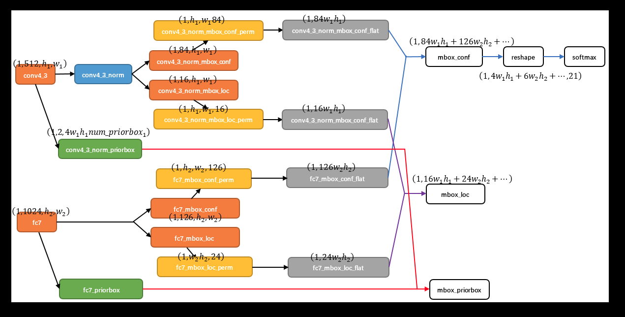
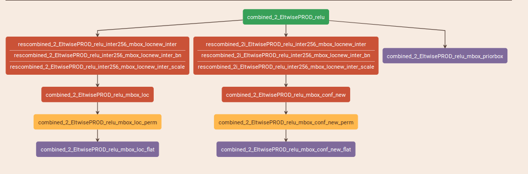
一个预测层的网络结构如下所示：

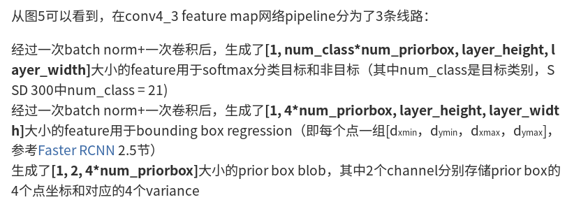
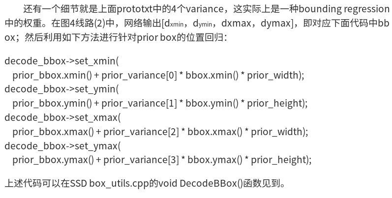
可以看到，是由三个分支组成的，分别是"PriorBox"层，以及conf、loc的预测层，其中，conf与loc的预测层的参数是由PriorBox的参数计算得到的，具体计算公式如下：

min_size与max_size分别对应一个尺度的预测框（有几个就对应几个预测框），in_size只管自己的预测，而max_size是与aspect_ratio联系在一起的；

filp参数是对应aspect_ratio的预测框*2，以几个max_size，再乘以几；最终得到结果为A

conf、loc的参数是在A的基础上再乘以类别数（加背景），以及4

如下，是需要预测两类的其中一个尺度的网络参数；

如上算出的是，每个格子需要预测的conf以及loc的个数；

每个预测层有H*W个格子，因此，总共预测的loc以及conf的个数是需要乘以H*W的；

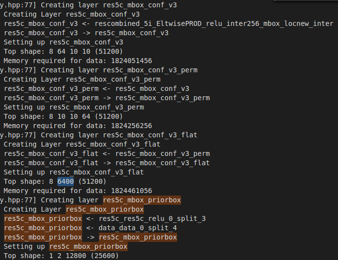
如下是某一个层的例子（转自：http://www.360doc.com/content/17/1013/16/42392246_694639090.shtml）

注意最后这里的num_priorbox的值与前面的并不一样，这里是每个预测层所有的输出框的个数：

layer {
  name: "combined_2_EltwisePROD_relu"
  type: "ReLU"
  bottom: "combined_2_EltwisePROD"
  top: "combined_2_EltwisePROD_relu"
}
###########################################
###################################################################

layer {
  name: "rescombined_2_EltwisePROD_relu_inter256_mbox_locnew_inter"
  type: "Convolution"
  bottom: "combined_2_EltwisePROD_relu"
  top: "rescombined_2_EltwisePROD_relu_inter256_mbox_locnew_inter"
  param {
    lr_mult:
    decay_mult:
  }
  convolution_param {
    num_output:
    bias_term: false
    pad:
    kernel_size:
    stride:
    weight_filler {
      type: "gaussian"
      std: 0.01
    }
  }
}
layer {
  name: "rescombined_2_EltwisePROD_relu_inter256_mbox_locnew_inter_bn"
  type: "BatchNorm"
  bottom: "rescombined_2_EltwisePROD_relu_inter256_mbox_locnew_inter"
  top: "rescombined_2_EltwisePROD_relu_inter256_mbox_locnew_inter"
  param {
    lr_mult:
    decay_mult:
  }
  param {
    lr_mult:
    decay_mult:
  }
  param {
    lr_mult:
    decay_mult:
  }
  batch_norm_param {
    moving_average_fraction: 0.999
    eps: 0.001
  }
}
layer {
  name: "rescombined_2_EltwisePROD_relu_inter256_mbox_locnew_inter_scale"
  type: "Scale"
  bottom: "rescombined_2_EltwisePROD_relu_inter256_mbox_locnew_inter"
  top: "rescombined_2_EltwisePROD_relu_inter256_mbox_locnew_inter"
  param {
    lr_mult:
    decay_mult:
  }
  param {
    lr_mult:
    decay_mult:
  }
  scale_param {
    filler {
      type: "constant"
      value: 1.0
    }
    bias_term: true
    bias_filler {
      type: "constant"
      value: 0.0
    }
  }
}

layer {
  name: "rescombined_2i_EltwisePROD_relu_inter256_mbox_locnew_inter"
  type: "Convolution"
  bottom: "combined_2_EltwisePROD_relu"
  top: "rescombined_2i_EltwisePROD_relu_inter256_mbox_locnew_inter"
  param {
    lr_mult:
    decay_mult:
  }
  convolution_param {
    num_output:
    bias_term: false
    pad:
    kernel_size:
    stride:
    weight_filler {
      type: "gaussian"
      std: 0.01
    }
  }
}
layer {
  name: "rescombined_2i_EltwisePROD_relu_inter256_mbox_locnew_inter_bn"
  type: "BatchNorm"
  bottom: "rescombined_2i_EltwisePROD_relu_inter256_mbox_locnew_inter"
  top: "rescombined_2i_EltwisePROD_relu_inter256_mbox_locnew_inter"
  param {
    lr_mult:
    decay_mult:
  }
  param {
    lr_mult:
    decay_mult:
  }
  param {
    lr_mult:
    decay_mult:
  }
  batch_norm_param {
    moving_average_fraction: 0.999
    eps: 0.001
  }
}
layer {
  name: "rescombined_2i_EltwisePROD_relu_inter256_mbox_locnew_inter_scale"
  type: "Scale"
  bottom: "rescombined_2i_EltwisePROD_relu_inter256_mbox_locnew_inter"
  top: "rescombined_2i_EltwisePROD_relu_inter256_mbox_locnew_inter"
  param {
    lr_mult:
    decay_mult:
  }
  param {
    lr_mult:
    decay_mult:
  }
  scale_param {
    filler {
      type: "constant"
      value: 1.0
    }
    bias_term: true
    bias_filler {
      type: "constant"
      value: 0.0
    }
  }
}

layer {
  name: "combined_2_EltwisePROD_relu_mbox_loc"
  type: "Convolution"
  bottom: "rescombined_2_EltwisePROD_relu_inter256_mbox_locnew_inter"
  top: "combined_2_EltwisePROD_relu_mbox_loc"
  param {
    lr_mult:
    decay_mult:
  }
  param {
    lr_mult:
    decay_mult:
  }
  convolution_param {
    engine: CAFFE
    num_output:
    pad:
    kernel_size:
    stride:
    weight_filler {
      type: "xavier"
    }
    bias_filler {
      type: "constant"
      value:
    }
  }
}
layer {
  name: "combined_2_EltwisePROD_relu_mbox_loc_perm"
  type: "Permute"
  bottom: "combined_2_EltwisePROD_relu_mbox_loc"
  top: "combined_2_EltwisePROD_relu_mbox_loc_perm"
  permute_param {
    order:
    order:
    order:
    order:
  }
}
layer {
  name: "combined_2_EltwisePROD_relu_mbox_loc_flat"
  type: "Flatten"
  bottom: "combined_2_EltwisePROD_relu_mbox_loc_perm"
  top: "combined_2_EltwisePROD_relu_mbox_loc_flat"
  flatten_param {
    axis:
  }
}
layer {
  name: "combined_2_EltwisePROD_relu_mbox_conf_new"
  type: "Convolution"
  bottom: "rescombined_2i_EltwisePROD_relu_inter256_mbox_locnew_inter"
  top: "combined_2_EltwisePROD_relu_mbox_conf_new"
  param {
    lr_mult:
    decay_mult:
  }
  param {
    lr_mult:
    decay_mult:
  }
  convolution_param {
    engine: CAFFE
    num_output:
    pad:
    kernel_size:
    stride:
    weight_filler {
      type: "xavier"
    }
    bias_filler {
      type: "constant"
      value:
    }
  }
}
layer {
  name: "combined_2_EltwisePROD_relu_mbox_conf_new_perm"
  type: "Permute"
  bottom: "combined_2_EltwisePROD_relu_mbox_conf_new"
  top: "combined_2_EltwisePROD_relu_mbox_conf_new_perm"
  permute_param {
    order:
    order:
    order:
    order:
  }
}
layer {
  name: "combined_2_EltwisePROD_relu_mbox_conf_new_flat"
  type: "Flatten"
  bottom: "combined_2_EltwisePROD_relu_mbox_conf_new_perm"
  top: "combined_2_EltwisePROD_relu_mbox_conf_new_flat"
  flatten_param {
    axis:
  }
}
layer {
  name: "combined_2_EltwisePROD_relu_mbox_priorbox"
  type: "PriorBox"
  bottom: "combined_2_EltwisePROD_relu"
  bottom: "data"
  top: "combined_2_EltwisePROD_relu_mbox_priorbox"
  prior_box_param {
    min_size: 12.0
    min_size: 6.0
    max_size: 30.0
    max_size: 20.0
    aspect_ratio:
    aspect_ratio: 2.5
    aspect_ratio:
    flip: true
    clip: false
    variance: 0.1
    variance: 0.1
    variance: 0.2
    variance: 0.2
    step:
    offset: 0.5
  }
}