分位数回归及其Python源码

天朗气清，惠风和畅。赋闲在家，正宜读书。前人文章，不得其解。代码开源，无人注释。你们不来，我行我上。废话少说，直入主题。o(￣︶￣)o

我们要探测自变量 $y$ 与因变量 $x$ 的关系，最简单的方法是线性回归，即假设：

$y_{i} = \beta_{0} + \beta_{1} x_{i} + e_{i}, i=1,...,n$

我们通过最小二乘方法 (OLS: ordinary least squares)， $\tilde{\beta_{1}}$ 的可靠性问题，我们同时对残差 $e_{i}$ 做了假设，即： $e_{i}$ 为均值为0，方差恒定的独立随机变量。 $\tilde{y_{i}} =\tilde{\beta_{0}} + \tilde{\beta_{1}}x_{i}$ 即为给定自变量 $x_{i}$ 下，因变量 $y_{i}$ 的条件均值。

假如残差 $e_{i}$ 不满足我们的假设，或者更重要地，我们不仅仅想要知道 $y_{i}$ 的在给定 $x_{i}$ 下的条件均值，而且想知道是条件中位数（更一般地，条件分位数），那么OLS下的线性回归就不能满足我们的需求。分位数回归(Quantile Regression)[2]解决了这些问题，下面我先给出一个分位数回归的实际应用例子，再简述其原理，最后再分析其在Python实现的源代码。

1. 一个例子：收入与食品消费

这个例子出自statasmodels:Quantile Regression.[3] 我们想探索家庭收入与食品消费的关系，数据出自working class Belgian households in 1857 (the Engel data).我们用Python包statsmodels实现分位数回归。

1.1 预处理

%matplotlib inline

import numpy as np

import pandas as pd

import statsmodels.api as sm

import statsmodels.formula.api as smf

import matplotlib.pyplot as plt

data = sm.datasets.engel.load_pandas().data

data.head()

	income	        foodexp

0	420.157651	255.839425

1	541.411707	310.958667

2	901.157457	485.680014

3	639.080229	402.997356

4	750.875606	495.560775

1.2 中位数回归（分位数回归的特例，q=0.5）

mod = smf.quantreg('foodexp ~ income', data)

res = mod.fit(q=.5)

print(res.summary())

                         QuantReg Regression Results

==============================================================================

Dep. Variable:                foodexp   Pseudo R-squared:               0.6206

Model:                       QuantReg   Bandwidth:                       64.51

Method:                 Least Squares   Sparsity:                        209.3

Date:                Mon, 21 Oct 2019   No. Observations:                  235

Time:                        17:46:59   Df Residuals:                      233

                                        Df Model:                            1

==============================================================================

                 coef    std err          t      P>|t|      [0.025      0.975]

------------------------------------------------------------------------------

Intercept     81.4823     14.634      5.568      0.000      52.649     110.315

income         0.5602      0.013     42.516      0.000       0.534       0.586

==============================================================================

The condition number is large, 2.38e+03. This might indicate that there are

strong multicollinearity or other numerical problems.

由结果可以知道 $foodexp_{median}=81.4623 + 0.5602income$ ，如何得到回归系数的估计？结果中的std err, t, Pseudo R-squared等是什么？我会在稍后解释。

1.3 数据可视化

我们先拟合10个分位数回归，分位数q分别在0.05到0.95之间。

quantiles = np.arange(.05, .96, .1)

def fit_model(q):

    res = mod.fit(q=q)

    return [q, res.params['Intercept'], res.params['income']] + \

            res.conf_int().loc['income'].tolist()

models = [fit_model(x) for x in quantiles]

models = pd.DataFrame(models, columns=['q', 'a', 'b', 'lb', 'ub'])

ols = smf.ols('foodexp ~ income', data).fit()

ols_ci = ols.conf_int().loc['income'].tolist()

ols = dict(a = ols.params['Intercept'],

           b = ols.params['income'],

           lb = ols_ci[0],

           ub = ols_ci[1])

print(models)

print(ols)

      q           a         b        lb        ub

0  0.05  124.880096  0.343361  0.268632  0.418090

1  0.15  111.693660  0.423708  0.382780  0.464636

2  0.25   95.483539  0.474103  0.439900  0.508306

3  0.35  105.841294  0.488901  0.457759  0.520043

4  0.45   81.083647  0.552428  0.525021  0.579835

5  0.55   89.661370  0.565601  0.540955  0.590247

6  0.65   74.033435  0.604576  0.582169  0.626982

7  0.75   62.396584  0.644014  0.622411  0.665617

8  0.85   52.272216  0.677603  0.657383  0.697823

9  0.95   64.103964  0.709069  0.687831  0.730306

{'a': 147.47538852370562, 'b': 0.48517842367692354, 'lb': 0.4568738130184233,

这里拟合了10个回归，其中q是对应的分位数，a是斜率，b是回归系数。lb和ub分别是b的95%置信区间的下界与上界。

现在来画出这10条回归线：

x = np.arange(data.income.min(), data.income.max(), 50)

get_y = lambda a, b: a + b * x

fig, ax = plt.subplots(figsize=(8, 6))

for i in range(models.shape[0]):

    y = get_y(models.a[i], models.b[i])

    ax.plot(x, y, linestyle='dotted', color='grey')

y = get_y(ols['a'], ols['b'])

ax.plot(x, y, color='red', label='OLS')

ax.scatter(data.income, data.foodexp, alpha=.2)

ax.set_xlim((240, 3000))

ax.set_ylim((240, 2000))

legend = ax.legend()

ax.set_xlabel('Income', fontsize=16)

ax.set_ylabel('Food expenditure', fontsize=16);

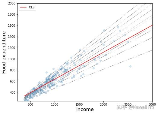
上图中虚线是分位数回归线，红线是线性最小二乘（OLS）的回归线。通过观察，我们可以发现3个现象:

随着收入提高，食品消费也在提高。
随着收入提高，家庭间食品消费的差别拉大。穷人别无选择，富人能选择生活方式，有喜欢吃贵的，也有喜欢吃便宜的。然而我们无法通过OLS发现这个现象，因为它只给了我们一个均值。
对与穷人来说，OLS预测值过高。这是因为少数的富人拉高了整体的均值，可见OLS对异常点敏感，不是一个稳健的模型。

2.分位数回归的原理

这部分是数理统计的内容，只关心如何实现的朋友可以略过。我们要解决以下这几个问题：

什么是分位数？
如何求分位数？
什么是分位数回归？
分位数回归的回归系数如何求得？
回归系数的检验如何进行？
如何评估回归拟合优度？

2.1 分位数的定义]

$Y$ 是随机变量， $Y$ 的累积密度函数是 $F_{y}(y) = P(Y\leq y)$ . $Y$ 的 $q$ 分位数为：

$Y_{q} =F_{Y}^{-1}(q)=inf\left\{ y:F_{Y} (y)\geq q\right\}$ , $q\in(0,1)$

假设有100个人，95%的人身高少于1.9m, 1.9m就是身高的95%分位数。

2.2 分位数的求法

$\tilde{Y_{q}} = argmin_{y_{q}}\sum_{i=1}^{n}{\rho_{q}(y_{i}-y_{q}}) =argmin_{y_{q}}[(q-1)\sum_{y_{i}<y{q}}^{}{(y_{i}-y_{q})+q\sum_{y_{i}\geq y_{q}}^{}{(y_{i}-y_{q)}}]}$

通过选择不同的 $y_{q}$ 值，使 $(q-1)\sum_{y_{i}<y{q}}^{}{(y_{i}-y_{q})+q\sum_{y_{i}\geq y_{q}}^{}{(y_{i}-y_{q)}}}$ 最小，对应的 $y_{q}$ 值即为 $Y$ 的 $q$ 分位数的估计 $\tilde{Y_{q}}$ .

2.3 分位数回归

对于OLS, 我们有：

$\tilde{Y}|X=X\tilde{\beta}$

$\tilde{\beta}$ 为 $||Y-X\beta||^{2}$ 最小化所对应的 $\beta$ ，类比地，对于 $q$ 分位数回归，我们有：

$\tilde{Y_{q}}|X=X\tilde{\beta_{q}}$

$\tilde{\beta_{q}}$ 为最小化：

$||\rho_{q}(Y-X\beta)||$ 即最小化 $\sum_{i=1}^{n}{\rho_{q}(y_{i}-x_{i}'\beta})=\sum_{i=1}^{n}[{(q-1)\sum_{y_{i}<x_{i}’\beta}^{}({y_{i}-x_{i}'\beta)+q\sum_{y_{i}\geq x_{i}\beta}^{}{(y_{i}-x_{i}'\beta)]}}}$

所对应的 $\beta$

2.4 系数估计

由于 $||\rho_{q}(Y-X\beta)||$ 不能直接对 $\beta$ 求导，我们只能用迭代的方法来逼近 $||\rho_{q}(Y-X\beta)||$ 最小时对应的 $\beta$ 值。statsmodels采用了Iteratively reweighted least squares （IRLS）的方法。

假设我们要求 $\beta$ 最小化形如下的 $L^{p}$ 范数：

$argmin_{\beta}||Y-X\beta||_{p}=argmin_{\beta}\sum_{i=1}^{n}{|y_{i}-x_{i}'\beta}|^{p}$

则第t+1步迭代的 $\beta$ 值为：

$\beta^{t+1}=argmin_{\beta}\sum_{i=1}^{n}{w_{i}^{(t)}}|y_{i}-x_{i}'\beta|^{2}=(X^{T}W^{(t)}X)^{-1}X^{T}W^{(t)}y$

$W^{t}$ 是对角矩阵且初始值为 $w_{i}^{(0)}=1$

第t次迭代 $w_{i}^{(t)}=|y_{i}-x_{i}'\beta|^{p-2}$

以中位数回归为例子(q=0.5),我们求：

$argmin_{\beta}\sum_{i=1}^{n}[{(q-1)\sum_{y_{i}<x_{i}'\beta}^{}({y_{i}-x_{i}'\beta)+q\sum_{y_{i}\geq x_{i}'\beta}^{}{(y_{i}-x_{i}'\beta)]}}}$

即 $argmin_{\beta}\sum_{i=1}^{n}[{-0.5\sum_{y_{i}<x_{i}'\beta}^{}({y_{i}-x_{i}'\beta)+0.5\sum_{y_{i}\geq x_{i}'\beta}^{}{(y_{i}-x_{i}'\beta)]}}}=argmin_{\beta}\sum_{i=1}^{n}{|y_{i}-x_{i}'\beta|}$

即最小化形如上的 $L^{1}$ 范数， $w_{i}^{(t)}=|y_{i}-x_{i}'\beta|^{-1}$

为避免分母为0，我们取 $w_{i}^{(t)}=1/max({{\delta,|y_{i}-x_{i}'\beta|}})$ , $\delta$ 是一个很小的数，例如0.0001.

2.5 回归系数的检验

我们通过2.4，多次迭代得出 $\beta$ 的估计值，为了得到假设检验的t统计量，我们只需得到 $\beta$ 的方差的估计。

$q$ 分位数回归 $\beta_{q}$ 的协方差矩阵的渐近估计为：

$Est.Asy.Var[\beta_{q}]=(X'X)^{-1}X'DX(X'X)^{-1}$

其中 $D$ 是对角矩阵，

当 $y_{i}>x_{i}'\beta$ , $d_{i}=[\frac{q}{f(0)}]^{2}$ , 当 $y_{i}\leq x_{i}'\beta$ ， $d_{i}=[\frac{1-q}{f(0)}]^{2}$

$f(0)$ 的估计为 $\tilde{f(0)}=\frac{1}{n}\sum_{i=1}^{n}{\frac{1}{h}K[\frac{e_{i}}{h}}]$

其中 $e_{i}=y_{i}-x_{i}'\beta$

$K()$ 为核函数（Kernel），可取Epa,Gaussian等. $h$ 为根据Stata 12所选的窗宽(bandwidth)[5]

回归结果中的std err即由 $Est.Asy.Var[\beta_{q}]$ 获得，t统计量等于 $\tilde{\beta}/\tilde{Var(\beta)}$ 。

2.6 拟合优度

对于OLS,我们用 $R^{2}=1-\frac{\sum_{i=1}^{n}{(y_{i}-\tilde{y_{i}})^{2}}}{\sum_{i=1}^{n}{(y_{i}-\bar{y_{i}}})^{2}}$ 来衡量拟合优度。对于 $q$ 分位数回归，我们类比得到：

$R_{q}^{2}=1-\frac{\sum_{i=1}^{n}{\rho_{q}(y_{i}-x_{i}'\beta})}{\sum_{i=1}^{n}{\rho_{q}(y_{i}-y_{q}})}$ ,其中 $y_{q}$ 为所有 $y$ 观察值的 $q$ 分位数。 $R_{q}^{2}$ 即为回归结果中的Pseudo R-squared。

3.Python源码分析

实现分位数回归的完整源码在，里面主要含有两个类QuantReg 和 QuantRegResults. 其中QuantReg是核心，包含了回归系数估计，协方差计算等过程。QuantRegResults计算拟合优度并组织回归结果。

3.1 QuantReg类

  #QuantReg是包中RegressionModel的一个子类

  class QuantReg(RegressionModel):

    #计算回归系数及其协方差矩阵。q是分位数，vcov是协方差矩阵，默认robust即2.5的方法。核函数kernel默认

    #epa,窗宽bandwidth默认hsheather.IRLS最大迭代次数默认1000，差值默认小于1e-6时停止迭代

    def fit(self, q=.5, vcov='robust', kernel='epa', bandwidth='hsheather',

            max_iter=1000, p_tol=1e-6, **kwargs):

        """

        Solve by Iterative Weighted Least Squares

        Parameters

        ----------

        q : float

            Quantile must be between 0 and 1

        vcov : str, method used to calculate the variance-covariance matrix

            of the parameters. Default is ``robust``:

            - robust : heteroskedasticity robust standard errors (as suggested

              in Greene 6th edition)

            - iid : iid errors (as in Stata 12)

        kernel : str, kernel to use in the kernel density estimation for the

            asymptotic covariance matrix:

            - epa: Epanechnikov

            - cos: Cosine

            - gau: Gaussian

            - par: Parzene

        bandwidth : str, Bandwidth selection method in kernel density

            estimation for asymptotic covariance estimate (full

            references in QuantReg docstring):

            - hsheather: Hall-Sheather (1988)

            - bofinger: Bofinger (1975)

            - chamberlain: Chamberlain (1994)

        """

        if q < 0 or q > 1:

            raise Exception('p must be between 0 and 1')

        kern_names = ['biw', 'cos', 'epa', 'gau', 'par']

        if kernel not in kern_names:

            raise Exception("kernel must be one of " + ', '.join(kern_names))

        else:

            kernel = kernels[kernel]

        if bandwidth == 'hsheather':

            bandwidth = hall_sheather

        elif bandwidth == 'bofinger':

            bandwidth = bofinger

        elif bandwidth == 'chamberlain':

            bandwidth = chamberlain

        else:

            raise Exception("bandwidth must be in 'hsheather', 'bofinger', 'chamberlain'")

        #endog样本因变量，exog样本自变量

        endog = self.endog

        exog = self.exog

        nobs = self.nobs

        exog_rank = np.linalg.matrix_rank(self.exog)

        self.rank = exog_rank

        self.df_model = float(self.rank - self.k_constant)

        self.df_resid = self.nobs - self.rank

        #IRLS初始化

        n_iter = 0

        xstar = exog

        beta = np.ones(exog_rank)

        # TODO: better start, initial beta is used only for convergence check

        # Note the following does not work yet,

        # the iteration loop always starts with OLS as initial beta

        # if start_params is not None:

        #    if len(start_params) != rank:

        #       raise ValueError('start_params has wrong length')

        #       beta = start_params

        #    else:

        #       # start with OLS

        #       beta = np.dot(np.linalg.pinv(exog), endog)

        diff = 10

        cycle = False

        history = dict(params = [], mse=[])

        #IRLS迭代

        while n_iter < max_iter and diff > p_tol and not cycle:

            n_iter += 1

            beta0 = beta

            xtx = np.dot(xstar.T, exog)

            xty = np.dot(xstar.T, endog)

            beta = np.dot(pinv(xtx), xty)

            resid = endog - np.dot(exog, beta)

            mask = np.abs(resid) < .000001

            resid[mask] = ((resid[mask] >= 0) * 2 - 1) * .000001

            resid = np.where(resid < 0, q * resid, (1-q) * resid)

            resid = np.abs(resid)

            #1/resid[:, np.newaxis]为更新权重W

            xstar = exog / resid[:, np.newaxis]

            diff = np.max(np.abs(beta - beta0))

            history['params'].append(beta)

            history['mse'].append(np.mean(resid*resid))

            #检查是否收敛，若收敛则提前停止迭代

            if (n_iter >= 300) and (n_iter % 100 == 0):

                # check for convergence circle, should not happen

                for ii in range(2, 10):

                    if np.all(beta == history['params'][-ii]):

                        cycle = True

                        warnings.warn("Convergence cycle detected", ConvergenceWarning)

                        break

        if n_iter == max_iter:

            warnings.warn("Maximum number of iterations (" + str(max_iter) +

                          ") reached.", IterationLimitWarning)

        #计算协方差矩阵

        e = endog - np.dot(exog, beta)

        # Greene (2008, p.407) writes that Stata 6 uses this bandwidth:

        # h = 0.9 * np.std(e) / (nobs**0.2)

        # Instead, we calculate bandwidth as in Stata 12

        iqre = stats.scoreatpercentile(e, 75) - stats.scoreatpercentile(e, 25)

        h = bandwidth(nobs, q)

        h = min(np.std(endog),

                iqre / 1.34) * (norm.ppf(q + h) - norm.ppf(q - h))

        fhat0 = 1. / (nobs * h) * np.sum(kernel(e / h))

        if vcov == 'robust':

            d = np.where(e > 0, (q/fhat0)**2, ((1-q)/fhat0)**2)

            xtxi = pinv(np.dot(exog.T, exog))

            xtdx = np.dot(exog.T * d[np.newaxis, :], exog)

            vcov = chain_dot(xtxi, xtdx, xtxi)

        elif vcov == 'iid':

            vcov = (1. / fhat0)**2 * q * (1 - q) * pinv(np.dot(exog.T, exog))

        else:

            raise Exception("vcov must be 'robust' or 'iid'")

        #用系数估计值和协方差矩阵创建一个QuantResults对象，并输出结果

        lfit = QuantRegResults(self, beta, normalized_cov_params=vcov)

        lfit.q = q

        lfit.iterations = n_iter

        lfit.sparsity = 1. / fhat0

        lfit.bandwidth = h

        lfit.history = history

        return RegressionResultsWrapper(lfit)

#核函数表达式

def _parzen(u):

    z = np.where(np.abs(u) <= .5, 4./3 - 8. * u**2 + 8. * np.abs(u)**3,

                 8. * (1 - np.abs(u))**3 / 3.)

    z[np.abs(u) > 1] = 0

    return z

kernels = {}

kernels['biw'] = lambda u: 15. / 16 * (1 - u**2)**2 * np.where(np.abs(u) <= 1, 1, 0)

kernels['cos'] = lambda u: np.where(np.abs(u) <= .5, 1 + np.cos(2 * np.pi * u), 0)

kernels['epa'] = lambda u: 3. / 4 * (1-u**2) * np.where(np.abs(u) <= 1, 1, 0)

kernels['gau'] = lambda u: norm.pdf(u)

kernels['par'] = _parzen

#kernels['bet'] = lambda u: np.where(np.abs(u) <= 1, .75 * (1 - u) * (1 + u), 0)

#kernels['log'] = lambda u: logistic.pdf(u) * (1 - logistic.pdf(u))

#kernels['tri'] = lambda u: np.where(np.abs(u) <= 1, 1 - np.abs(u), 0)

#kernels['trw'] = lambda u: 35. / 32 * (1 - u**2)**3 * np.where(np.abs(u) <= 1, 1, 0)

#kernels['uni'] = lambda u: 1. / 2 * np.where(np.abs(u) <= 1, 1, 0)

#窗宽计算

def hall_sheather(n, q, alpha=.05):

    z = norm.ppf(q)

    num = 1.5 * norm.pdf(z)**2.

    den = 2. * z**2. + 1.

    h = n**(-1. / 3) * norm.ppf(1. - alpha / 2.)**(2./3) * (num / den)**(1./3)

    return h

def bofinger(n, q):

    num = 9. / 2 * norm.pdf(2 * norm.ppf(q))**4

    den = (2 * norm.ppf(q)**2 + 1)**2

    h = n**(-1. / 5) * (num / den)**(1. / 5)

    return h

def chamberlain(n, q, alpha=.05):

    return norm.ppf(1 - alpha / 2) * np.sqrt(q*(1 - q) / n)

3.2 QuantRegResults类

这里我只给出计算拟合优度的代码。

class QuantRegResults(RegressionResults):

    '''Results instance for the QuantReg model'''

    @cache_readonly

    def prsquared(self):

        q = self.q

        endog = self.model.endog

        #e为残差

        e = self.resid

        e = np.where(e < 0, (1 - q) * e, q * e)

        e = np.abs(e)

        ered = endog - stats.scoreatpercentile(endog, q * 100)

        ered = np.where(ered < 0, (1 - q) * ered, q * ered)

        ered = np.abs(ered)

        return 1 - np.sum(e) / np.sum(ered)

4.总结

上文我先给出了一个分位数回归的应用例子，进而叙述了分位数回归的原理，最后再分析了Python实现的源码。

分位数回归对比起OLS回归，虽然较为复杂，但它有三个主要优势：

能反映因变量分位数与自变量的关系，而不仅仅反映因变量均值与自变量的关系。
分位数回归对残差不作任何假设。
分位数回归受异常点的影响较小。

参考

^https://en.wikipedia.org/wiki/Ordinary_least_squares
^QUANTILE REGRESSION http://www.econ.uiuc.edu/~roger/research/rq/rq.pdf
^https://www.statsmodels.org/dev/examples/notebooks/generated/quantile_regression.html
^[1](https://www.zhihu.com/#ref_4_0)b c https://en.wikipedia.org/wiki/Quantile_regression
^[2](https://www.zhihu.com/#ref_5_0)b c https://www.statsmodels.org/devel/_modules/statsmodels/regression/quantile_regression.html
^https://en.wikipedia.org/wiki/Iteratively_reweighted_least_squares
^Green,W. H. (2008). Econometric Analysis. Sixth Edition. International Student Edition.
^https://www.ibm.com/support/knowledgecenter/en/SSLVMB_sub/statistics_mainhelp_ddita/spss/regression/idh_quantile.html

a ↩︎
a ↩︎