Instance Segmentation with Mask R-CNN and TensorFlow

Back in November, we open-sourced our implementation of Mask R-CNN, and since then it’s been forked 1400 times, used in a lot of projects, and improved upon by many generous contributors. We received a lot of questions as well, so in this post I’ll explain how the model works and show how to use it in a real application.

I’ll cover two things: First, an overview of Mask RCNN. And, second, how to train a model from scratch and use it to build a smart color splash filter.

Code Tip:
We’re sharing the code here. Including the dataset I built and the trained model. Follow along!

What is Instance Segmentation?

Instance segmentation is the task of identifying object outlines at the pixel level. Compared to similar computer vision tasks, it’s one of the hardest possible vision tasks. Consider the following asks:

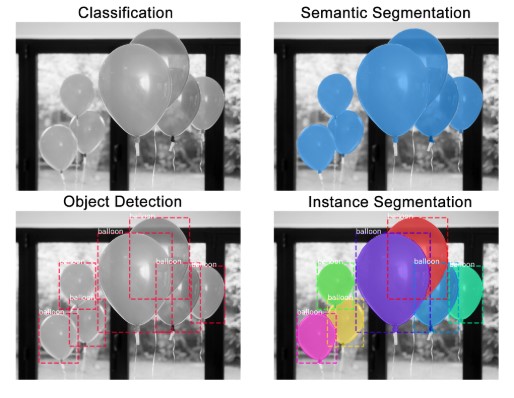
• Classification: There is a balloon in this image.
• Semantic Segmentation: These are all the balloon pixels.
• Object Detection: There are 7 balloons in this image at these locations. We’re starting to account for objects that overlap.
• Instance Segmentation: There are 7 balloons at these locations, and these are the pixels that belong to each one.

Mask R-CNN

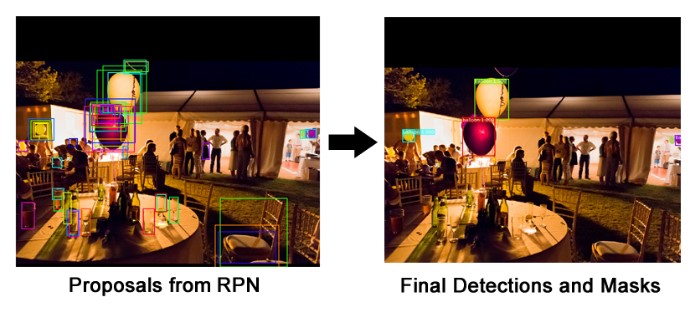
Mask R-CNN (regional convolutional neural network) is a two stage framework: the first stage scans the image and generates proposals(areas likely to contain an object). And the second stage classifies the proposals and generates bounding boxes and masks.

It was introduced last year via the Mask R-CNN paper to extend its predecessor, Faster R-CNN, by the same authors. Faster R-CNN is a popular framework for object detection, and Mask R-CNN extends it with instance segmentation, among other things.

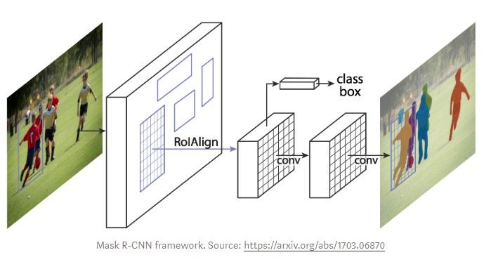
At a high level, Mask R-CNN consists of these modules:

1. Backbone

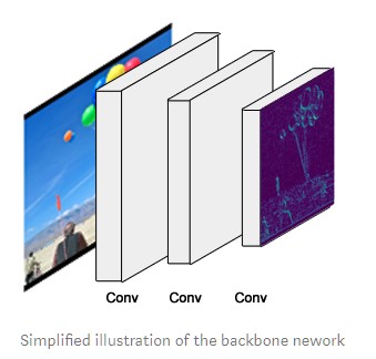
This is a standard convolutional neural network (typically, ResNet50 or ResNet101) that serves as a feature extractor. The early layers detect low level features (edges and corners), and later layers successively detect higher level features (car, person, sky).

Passing through the backbone network, the image is converted from 1024x1024px x 3 (RGB) to a feature map of shape 32x32x2048. This feature map becomes the input for the following stages.

Code Tip:
The backbone is built in the function resnet_graph(). The code supports ResNet50 and ResNet101.

Feature Pyramid Network

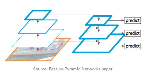
While the backbone described above works great, it can be improved upon. The Feature Pyramid Network (FPN) was introduced by the same authors of Mask R-CNN as an extension that can better represent objects at multiple scales.

FPN improves the standard feature extraction pyramid by adding a second pyramid that takes the high level features from the first pyramid and passes them down to lower layers. By doing so, it allows features at every level to have access to both, lower and higher level features.

Our implementation of Mask RCNN uses a ResNet101 + FPN backbone.

Code Tip:
The FPN is created in MaskRCNN.build(). The section after building the ResNet.
RPN introduces additional complexity: rather than a single backbone feature map in the standard backbone (i.e. the top layer of the first pyramid), in FPN there is a feature map at each level of the second pyramid. We pick which to use dynamically depending on the size of the object. I’ll continue to refer to the backbone feature map as if it’s one feature map, but keep in mind that when using FPN, we’re actually picking one out of several at runtime.

2. Region Proposal Network (RPN)

The RPN is a lightweight neural network that scans the image in a sliding-window fashion and finds areas that contain objects.

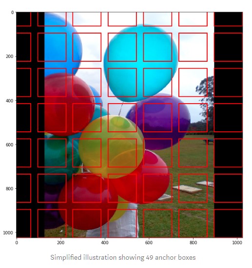
The regions that the RPN scans over are called anchors. Which are boxes distributed over the image area, as show on the left. This is a simplified view, though. In practice, there are about 200K anchors of different sizes and aspect ratios, and they overlap to cover as much of the image as possible.

How fast can the RPN scan that many anchors? Pretty fast, actually. The sliding window is handled by the convolutional nature of the RPN, which allows it to scan all regions in parallel (on a GPU). Further, the RPN doesn’t scan over the image directly (even though we draw the anchors on the image for illustration). Instead, the RPN scans over the backbone feature map. This allows the RPN to reuse the extracted features efficiently and avoid duplicate calculations. With these optimizations, the RPN runs in about 10 ms according to the Faster RCNN paper that introduced it. In Mask RCNN we typically use larger images and more anchors, so it might take a bit longer.

Code Tip:
The RPN is created in rpn_graph(). Anchor scales and aspect ratios are controlled by RPN_ANCHOR_SCALES and RPN_ANCHOR_RATIOS in config.py.

The RPN generates two outputs for each anchor:

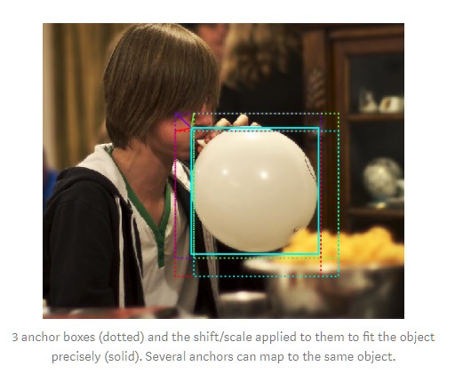
1. Anchor Class: One of two classes: foreground or background. The FG class implies that there is likely an object in that box.
2. Bounding Box Refinement: A foreground anchor (also called positive anchor) might not be centered perfectly over the object. So the RPN estimates a delta (% change in x, y, width, height) to refine the anchor box to fit the object better.

Using the RPN predictions, we pick the top anchors that are likely to contain objects and refine their location and size. If several anchors overlap too much, we keep the one with the highest foreground score and discard the rest (referred to as Non-max Suppression). After that we have the final proposals (regions of interest) that we pass to the next stage.

Code Tip:
The ProposalLayer is a custom Keras layer that reads the output of the RPN, picks top anchors, and applies bounding box refinement.

3. ROI Classifier & Bounding Box Regressor

This stage runs on the regions of interest (ROIs) proposed by the RPN. And just like the RPN, it generates two outputs for each ROI:

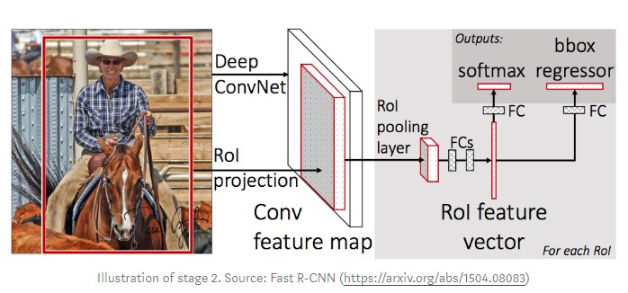
1. Class: The class of the object in the ROI. Unlike the RPN, which has two classes (FG/BG), this network is deeper and has the capacity to classify regions to specific classes (person, car, chair, …etc.). It can also generate a background class, which causes the ROI to be discarded.
2. Bounding Box Refinement: Very similar to how it’s done in the RPN, and its purpose is to further refine the location and size of the bounding box to encapsulate the object.

Code Tip:
The classifier and bounding box regressor are created in fpn_classifier_graph().

ROI Pooling

There is a bit of a problem to solve before we continue. Classifiers don’t handle variable input size very well. They typically require a fixed input size. But, due to the bounding box refinement step in the RPN, the ROI boxes can have different sizes. That’s where ROI Pooling comes into play.

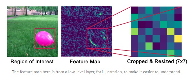
ROI pooling refers to cropping a part of a feature map and resizing it to a fixed size. It’s similar in principle to cropping part of an image and then resizing it (but there are differences in implementation details).

The authors of Mask R-CNN suggest a method they named ROIAlign, in which they sample the feature map at different points and apply a bilinear interpolation. In our implementation, we used TensorFlow’s crop_and_resize function for simplicity and because it’s close enough for most purposes.

Code Tip:
ROI pooling is implemented in the class PyramidROIAlign.

4. Segmentation Masks

If you stop at the end of the last section then you have a Faster R-CNN framework for object detection. The mask network is the addition that the Mask R-CNN paper introduced.

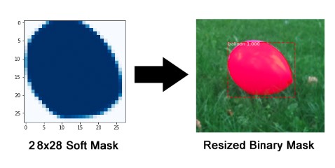
The mask branch is a convolutional network that takes the positive regions selected by the ROI classifier and generates masks for them. The generated masks are low resolution: 28x28 pixels. But they are soft masks, represented by float numbers, so they hold more details than binary masks. The small mask size helps keep the mask branch light. During training, we scale down the ground-truth masks to 28x28 to compute the loss, and during inferencing we scale up the predicted masks to the size of the ROI bounding box and that gives us the final masks, one per object.

Code Tip:
The mask branch is in build_fpn_mask_graph().

Let’s Build a Color Splash Filter

Unlike most image editing apps that include this filter, our filter will be a bit smarter: It finds the objects automatically. Which becomes even more useful if you want to apply it to videos rather than a single image.

Training Dataset

Typically, I’d start by searching for public datasets that contain the objects I need. But in this case, I wanted to document the full cycle and show how to build a dataset from scratch.

I searched for balloon images on flickr, limiting the license type to “Commercial use & mods allowed”. This returned more than enough images for my needs. I picked a total of 75 images and divided them into a training set and a validation set. Finding images is easy. Annotating them is the hard part.

Wait! Don’t we need, like, a million images to train a deep learning model? Sometimes you do, but often you don’t. I’m relying on two main points to reduce my training requirements significantly:

First, transfer learning. Which simply means that, instead of training a model from scratch, I start with a weights file that’s been trained on the COCO dataset (we provide that in the github repo). Although the COCO dataset does not contain a balloon class, it contains a lot of other images (~120K), so the trained weights have already learned a lot of the features common in natural images, which really helps. And, second, given the simple use case here, I’m not demanding high accuracy from this model, so the tiny dataset should suffice.

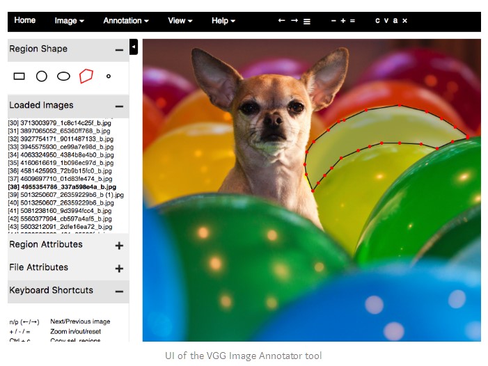
There are a lot of tools to annotate images. I ended up using VIA (VGG Image Annotator) because of its simplicity. It’s a single HTML file that you download and open in a browser. Annotating the first few images was very slow, but once I got used to the user interface, I was annotating at around an object a minute.

If you don’t like the VIA tool, here is a list of the other tools I tested:

• LabelMe: One of the most known tools. The UI was a bit too slow, though, especially when zooming in on large images.
• RectLabel: Simple and easy to work with. Mac only.
• LabelBox: Pretty good for larger labeling projects and has options for different types of labeling tasks.
• VGG Image Annotator (VIA): Fast, light, and really well designed. This is the one I ended up using.
• COCO UI: The tool used to annotate the COCO dataset.

Loading the Dataset

There isn’t a universally accepted format to store segmentation masks. Some datasets save them as PNG images, others store them as polygon points, and so on. To handle all these cases, our implementation provides a Dataset class that you inherit from and then override a few functions to read your data in whichever format it happens to be.

The VIA tool saves the annotations in a JSON file, and each mask is a set of polygon points. I didn’t find documentation for the format, but it’s pretty easy to figure out by looking at the generated JSON. I included comments in the code to explain how the parsing is done.

Code Tip:
An easy way to write code for a new dataset is to copy coco.py and modify it to your needs. Which is what I did. I saved the new file as balloons.py

My BalloonDataset class looks like this:

class BalloonDataset(utils.Dataset):
    def load_balloons(self, dataset_dir, subset):
        ...
    def load_mask(self, image_id):
        ...
    def image_reference(self, image_id):
        ...

load_balloons reads the JSON file, extracts the annotations, and iteratively calls the internal add_class and add_image functions to build the dataset.

load_mask generates bitmap masks for every object in the image by drawing the polygons.

image_reference simply returns a string that identifies the image for debugging purposes. Here it simply returns the path of the image file.

You might have noticed that my class doesn’t contain functions to load images or return bounding boxes. The default load_image function in the base Dataset class handles loading images. And, bounding boxes are generated dynamically from the masks.

Code Tip:
Your dataset might not be in JSON. My BalloonDataset class reads JSON because that’s what the VIA tool generates. Don’t convert your dataset to a format similar to COCO or the VIA format. Insetad, write your own Dataset class to load whichever format your dataset comes in. See the samples and notice how each uses its own Dataset class.

Verify the Dataset

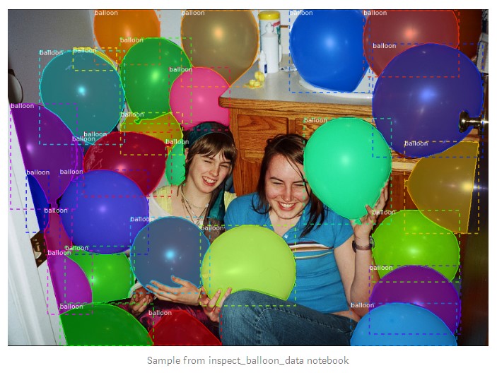
To verify that my new code is implemented correctly I added this Jupyter notebook. It loads the dataset, visualizes masks and bounding boxes, and visualizes the anchors to verify that my anchor sizes are a good fit for my object sizes. Here is an example of what you should expect to see:

Code Tip:
To create this notebook I copied inspect_data.ipynb, which we wrote for the COCO dataset, and modified one block of code at the top to load the Balloons dataset instead.

Configurations

The configurations for this project are similar to the base configuration used to train the COCO dataset, so I just needed to override 3 values. As I did with the Dataset class, I inherit from the base Config class and add my overrides:

class BalloonConfig(Config):
    # Give the configuration a recognizable name
    NAME = "balloons"
    # Number of classes (including background)
    NUM_CLASSES = 1 + 1  # Background + balloon
    # Number of training steps per epoch
    STEPS_PER_EPOCH = 100

The base configuration uses input images of size 1024x1024 px for best accuracy. I kept it that way. My images are a bit smaller, but the model resizes them automatically.

Code Tip:
The base Config class is in config.py. And BalloonConfig is inballoons.py.

Training

Mask R-CNN is a fairly large model. Especially that our implementation uses ResNet101 and FPN. So you need a modern GPU with 12GB of memory. It might work on less, but I haven’t tried. I used Amazon’s P2 instances to train this model, and given the small dataset, training takes less than an hour.

Start the training with this command, running from the balloon directory. Here, we’re specifying that training should start from the pre-trained COCO weights. The code will download the weights from our repository automatically:

python3 balloon.py train --dataset=/path/to/dataset --model=coco

And to resume training if it stopped:

python3 balloon.py train --dataset=/path/to/dataset --model=last

Code Tip:
In addition to balloons.py, the repository has three more examples: train_shapes.ipynb which trains a toy model to detect geometric shapes, coco.py which trains on the COCO dataset, and nucleus which segments nuclei in microscopy images.

Inspecting the Results

The inspect_balloon_model notebook shows the results generated by the trained model. Check the notebook for more visualizations and a step by step walk through the detection pipeline.

Code Tip:
This notebook is a simplified version of inspect_mode.ipynb, which includes visualizations and debugging code for the COCO dataset.

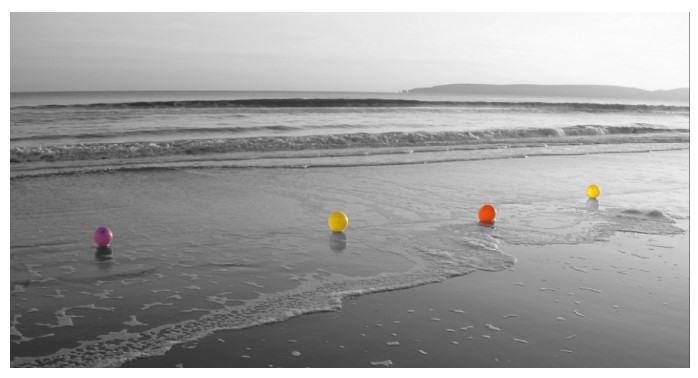
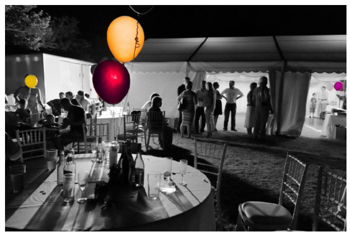
Color Splash

Finally, now that we have object masks, let’s use them to apply the color splash effect. The method is really simple: create a grayscale version of the image, and then, in areas marked by the object mask, copy back the color pixels from original image. Here is an example:

Code Tip:
The code that applies the effect is in the color_splash() function. And detect_and_color_splash() handles the whole process from loading the image, running instance segmentation, and applying the color splash filter.

FAQ

• Q: I want to dive deeper and understand the details, what should I read?
  A: Read these papers in this order: RCNN (pdf), Fast RCNN, Faster RCNN, FPN, Mask RCNN.
• Q: Where can I ask more questions?
  A: The Issues page on GitHub is active, you can use it for questions, as well as to report issues. Remember to search closed issues as well in case your question has been answered already.
• Q: Can I contribute to this project?
  A: That would be great. Pull Requests are always welcome.
• Q: Can I join your team and work on fun projects like this one?
  A: Yes, we’re hiring for deep learning and computer vision. Apply here.

 

 

 

来源： https://engineering.matterport.com/splash-of-color-instance-segmentation-with-mask-r-cnn-and-tensorflow-7c761e238b46