Exercise: PCA in 2D

Step 0: Load data

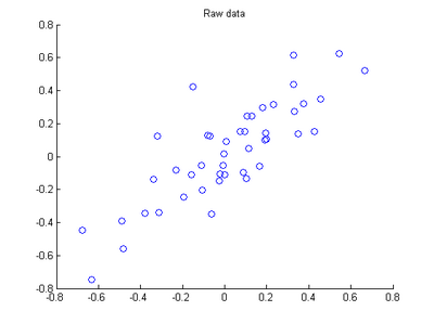
The starter code contains code to load 45 2D data points. When plotted using the scatter function, the results should look like the following:

Step 1: Implement PCA

In this step, you will implement PCA to obtain x_rot, the matrix in which the data is "rotated" to the basis comprising made up of the principal components

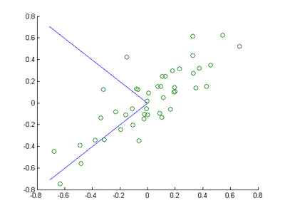
Step 1a: Finding the PCA basis

Find and , and draw two lines in your figure to show the resulting basis on top of the given data points.

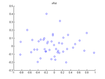
Step 1b: Check xRot

Compute xRot, and use the scatter function to check that xRot looks as it should, which should be something like the following:

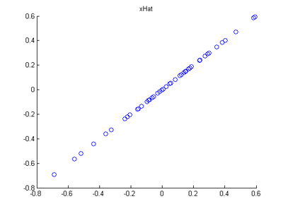
Step 2: Dimension reduce and replot

In the next step, set k, the number of components to retain, to be 1

Step 3: PCA Whitening

Step 4: ZCA Whitening

Code

close all

%%================================================================
%% Step : Load data
%  We have provided the code to load data from pcaData.txt into x.
%  x is a  *  matrix, where the kth column x(:,k) corresponds to
%  the kth data point.Here we provide the code to load natural image data into x.
%  You do not need to change the code below.

x = load('pcaData.txt','-ascii'); % 载入数据
figure();
scatter(x(, :), x(, :)); % 用圆圈绘制出数据分布
title('Raw data');

%%================================================================
%% Step 1a: Implement PCA to obtain U
%  Implement PCA to obtain the rotation matrix U, which is the eigenbasis
%  sigma. 

% -------------------- YOUR CODE HERE --------------------
u = zeros(size(x, )); % You need to compute this
[n m]=size(x);
% x=x-repmat(mean(x,),,m);  %预处理，均值为零 —— 2维，每一维减去该维上的均值
sigma=(1.0/m)*x*x'; % 协方差矩阵
[u s v]=svd(sigma);

% --------------------------------------------------------
hold on
plot([ u(,)], [ u(,)]); % 画第一条线
plot([ u(,)], [ u(,)]); % 画第二条线
scatter(x(, :), x(, :));
hold off

%%================================================================
%% Step 1b: Compute xRot, the projection on to the eigenbasis
%  Now, compute xRot by projecting the data on to the basis defined
%  by U. Visualize the points by performing a scatter plot.

% -------------------- YOUR CODE HERE --------------------
xRot = zeros(size(x)); % You need to compute this
xRot=u'*x;

% -------------------------------------------------------- 

% Visualise the covariance matrix. You should see a line across the
% diagonal against a blue background.
figure();
scatter(xRot(, :), xRot(, :));
title('xRot');

%%================================================================
%% Step : Reduce the number of dimensions from  to .
%  Compute xRot again (this time projecting to  dimension).
%  Then, compute xHat by projecting the xRot back onto the original axes
%  to see the effect of dimension reduction

% -------------------- YOUR CODE HERE --------------------
k = ; % Use k =  and project the data onto the first eigenbasis
xHat = zeros(size(x)); % You need to compute this
xHat = u*([u(:,),zeros(n,)]'*x); % 降维
% 使特征点落在特征向量所指的方向上而不是原坐标系上

% --------------------------------------------------------
figure();
scatter(xHat(, :), xHat(, :));
title('xHat');

%%================================================================
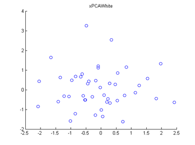
%% Step : PCA Whitening
%  Complute xPCAWhite and plot the results.

epsilon = 1e-;
% -------------------- YOUR CODE HERE --------------------
xPCAWhite = zeros(size(x)); % You need to compute this
xPCAWhite = diag(./sqrt(diag(s)+epsilon))*u'*x;  % 每个特征除以对应的特征向量，以使每个特征有一致的方差
% --------------------------------------------------------
figure();
scatter(xPCAWhite(, :), xPCAWhite(, :));
title('xPCAWhite');

%%================================================================
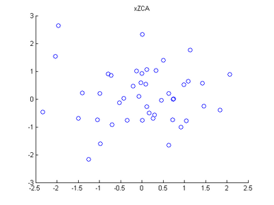
%% Step : ZCA Whitening
%  Complute xZCAWhite and plot the results.

% -------------------- YOUR CODE HERE --------------------
xZCAWhite = zeros(size(x)); % You need to compute this
xZCAWhite = u*diag(./sqrt(diag(s)+epsilon))*u'*x;

% --------------------------------------------------------
figure();
scatter(xZCAWhite(, :), xZCAWhite(, :));
title('xZCAWhite');

%% Congratulations! When you have reached this point, you are done!
%  You can now move onto the next PCA exercise. :)