Ceres 自动求导解析-从原理到实践

Ceres 自动求导解析-从原理到实践

1.0 前言

Ceres 有一个自动求导功能，只要你按照Ceres要求的格式写好目标函数，Ceres会自动帮你计算精确的导数（或者雅克比矩阵），这极大节约了算法开发者的时间，但是笔者在使用的时候一直觉得这是个黑盒子，特别是之前在做深度学习的时候，神经网络本事是一个很盒模型了，再加上 pytorch 的自动求导，简直是黑上加黑。现在转入视觉SLAM方向，又碰到了 Ceres 的自动求导，是时候揭开其真实的面纱了。知其然并知其所以然才是一名算法工程师应有的基本素养。

2.0 Ceres求导简介

Ceres 一共有三种求导的方式提供给开发者，分别是：

解析求导，也就是手动计算出导数的解析形式。

例如有如下函数;

\[y = \frac{b_1}{(1+e^{b_2-b_3x})^{1/b_4}}
\]

构建误差函数：

\[\begin{split}\begin{align}
E(b_1, b_2, b_3, b_4)
&= \sum_i f^2(b_1, b_2, b_3, b_4 ; x_i, y_i)\\
&= \sum_i \left(\frac{b_1}{(1+e^{b_2-b_3x_i})^{1/b_4}} - y_i\right)^2\\
\end{align}\end{split}
\]

对待优化变量的导数为：

\[\begin{split}\begin{align}
D_1 f(b_1, b_2, b_3, b_4; x,y) &= \frac{1}{(1+e^{b_2-b_3x})^{1/b_4}}\\
D_2 f(b_1, b_2, b_3, b_4; x,y) &=
\frac{-b_1e^{b_2-b_3x}}{b_4(1+e^{b_2-b_3x})^{1/b_4 + 1}} \\
D_3 f(b_1, b_2, b_3, b_4; x,y) &=
\frac{b_1xe^{b_2-b_3x}}{b_4(1+e^{b_2-b_3x})^{1/b_4 + 1}} \\
D_4 f(b_1, b_2, b_3, b_4; x,y) & = \frac{b_1 \log\left(1+e^{b_2-b_3x}\right) }{b_4^2(1+e^{b_2-b_3x})^{1/b_4}}
\end{align}\end{split}
\]
数值求导，当对变量增加一个微小的增量，然后观察此时的残差和原先残差的下降比例即可，其实就是导数的定义。

\[Df(x) = \lim_{h \rightarrow 0} \frac{f(x + h) - f(x)}{h}
\]

当然其实也有两种形式对导数进行数值上的近似，第一种是Forward Differences：

\[Df(x) \approx \frac{f(x + h) - f(x)}{h}
\]

第二种是 Central Differences：

\[Df(x) \approx \frac{f(x + h) - f(x - h)}{2h}
\]

Ceres 的官方文档上是认为第二种比第一种好的，但是其实官方还介绍了第三种，这里就不详说了，感兴趣的可以去看官方文档：Ridders’ Method。

这里有三种数值微分方法的效果对比，从右向左看：

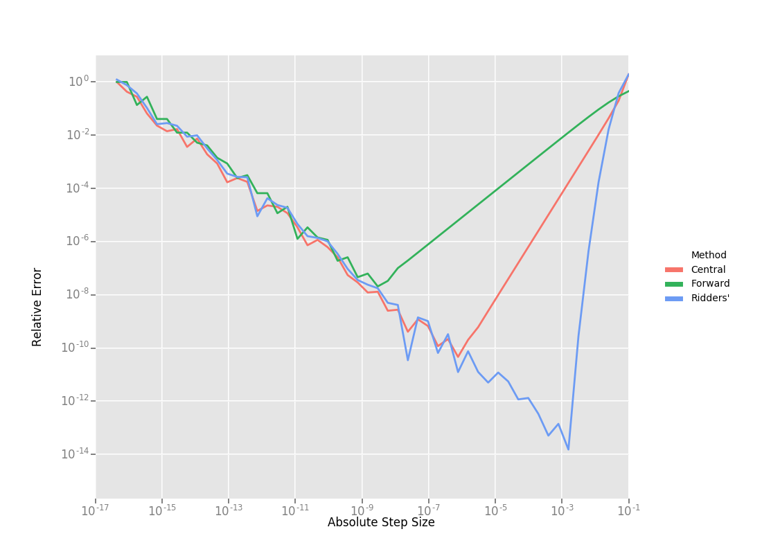
效果依次是 $Ridders > Central > Forwad$

第三种则是今天要介绍的主角，自动求导。

3.0 Ceres 自动求导原理

3.1 官方解释

其实官方对自动求导做出了解释，但是笔者觉得写的不够直观，比较抽象，不过既然是官方出品，还是非常有必要去看一看的。http://ceres-solver.org/automatic_derivatives.html。

3.2 自我理解

$\quad$这里笔者根据网上和官方的资料整理了一下自己的理解。Ceres 自动求导的核心是运算符的重载与Ceres自有的 Jet 变量。

举一个例子：

函数 $\mathrm{f}(\mathrm{x})=\mathrm{h}(\mathrm{x}) * \mathrm{~g}(\mathrm{x})$ , 他的目标函数值为 $\mathrm{h}(\mathrm{x}) * \mathrm{~g}(\mathrm{x})$ , 导数为

\[\mathrm{f}^{\prime}(\mathrm{x})=\mathrm{h}^{\prime}(\mathrm{x}) \mathrm{g}(\mathrm{x})+\mathrm{h}(\mathrm{x}) \mathrm{g}^{\prime}(\mathrm{x})
\]

其中 $h(x)$, $g(x)$ 都是标量函数.

如果我们定义一种数据类型,

\[Data \{ double\ \ value, double\ \ derived \}
\]

并且对于数据类型 Data，重载乘法运算符

\[data1*data2=\begin{bmatrix}
data1.value*data2.value \\
data1.derived*data2.value+data1.value*data2.derived
\end{bmatrix}
\]

令 $h(x) =[h(x),{h(x)}' ] , g(x)=[g(x),{g(x)' }]$。$f(x)=h(x) * g(x)$, 那么f_x.derived 就是$f(x)$的导数，f_x.value 即为$f(x)$的数值。value 储存变量的函数值, derived 储存变量对 $\mathrm{x}$ 的导数。类似，如果我们对数据类型 Data 重载所有可能用到的运算符. “$+- * / \log , \exp , \cdots$” 。那么在变量 $h(x),g(x)$经过任意次运算后，$result=h(x)+g(x)*h(x)+exp(h(x))…$, 任然能获得函数值 result.value 和他的导数值 result.derived，这就是Ceres 自动求导的原理。

上面讲的都是单一自变量的自动求导，对于多元函数$f(x_i)$。对于n 元函数，Data 里面的 double derived 就替换为 double* derived，derived[i] 为对于第i个自变量的导数值。

并且对于数据类型 Data，乘法运算符重载为

\[data1*data2=\begin{bmatrix}
data1.value*data2.value \\
derived[i]=data1.derived[i]*data2.value+data1.value*data2.derived[i]
\end{bmatrix}
\]

其余的运算符重载方法也做相应改变。这样对多元函数的自动求导问题也就解决了。Ceres 里面的Jet 数据类型类似于这里Data 类型，并且Ceres 对Jet 数据类型进行了几乎所有数学运算符的重载，以达到自动求导的目的。

4.0 实践

4.1 Jet 的实现

这里我们模仿 Ceres 实现了 Jet ，并准备了两个具体的示例程序，Jet 具体代码在 ceres_jet.hpp 中，包装成了一个头文件，在使用的时候进行调用即可。这里也包含了一个 ceres_rotation.hpp 的头文件，是为了我们的第二个例子实现。具体代码如下：

ceres_jet.hpp

#ifndef _CERES_JET_HPP__

#define _CERES_JET_HPP__

#include <math.h>

#include <stdio.h>

#include <eigen3/Eigen/Core>

#include <eigen3/Eigen/Dense>

#include <eigen3/Eigen/Sparse>

#include "eigen3/Eigen/Eigen"

#include "eigen3/Eigen/SparseQR"

#include <fstream>

#include <iostream>

#include <map>

#include <queue>

#include <set>

#include <vector>

#include "ceres_rotation.hpp"

#include "algorithm"

#include "stdlib.h"

template <int N>

struct jet

{

  Eigen::Matrix<double, N, 1> v;

  double a;

  jet() : a(0.0) {}

  jet(const double& value) : a(value) { v.setZero(); }

  EIGEN_STRONG_INLINE jet(const double& value,

                          const Eigen::Matrix<double, N, 1>& v_)

      : a(value), v(v_)

  {

  }

  jet(const double value, const int index)

  {

    v.setZero();

    a = value;

    v(index, 0) = 1.0;

  }

  void init(const double value, const int index)

  {

    v.setZero();

    a = value;

    v(index, 0) = 1.0;

  }

};

/****************jet overload******************/

// for the camera BA,the autodiff only need overload the operator :jet+jet

// number+jet -jet jet-number jet*jet number/jet jet/jet sqrt(jet) cos(jet)

// sin(jet)  +=(jet) overload jet + jet

template <int N>

inline jet<N> operator+(const jet<N>& A, const jet<N>& B)

{

  return jet<N>(A.a + B.a, A.v + B.v);

}  // end jet+jet

// overload number + jet

template <int N>

inline jet<N> operator+(double A, const jet<N>& B)

{

  return jet<N>(A + B.a, B.v);

}  // end number+jet

template <int N>

inline jet<N> operator+(const jet<N>& B, double A)

{

  return jet<N>(A + B.a, B.v);

}  // end number+jet

// overload jet-number

template <int N>

inline jet<N> operator-(const jet<N>& A, double B)

{

  return jet<N>(A.a - B, A.v);

}

// overload number * jet because jet *jet need A.a *B.v+B.a*A.v.So the number

// *jet is required

template <int N>

inline jet<N> operator*(double A, const jet<N>& B)

{

  return jet<N>(A * B.a, A * B.v);

}

template <int N>

inline jet<N> operator*(const jet<N>& A, double B)

{

  return jet<N>(B * A.a, B * A.v);

}

// overload -jet

template <int N>

inline jet<N> operator-(const jet<N>& A)

{

  return jet<N>(-A.a, -A.v);

}

template <int N>

inline jet<N> operator-(double A, const jet<N>& B)

{

  return jet<N>(A - B.a, -B.v);

}

template <int N>

inline jet<N> operator-(const jet<N>& A, const jet<N>& B)

{

  return jet<N>(A.a - B.a, A.v - B.v);

}

// overload jet*jet

template <int N>

inline jet<N> operator*(const jet<N>& A, const jet<N>& B)

{

  return jet<N>(A.a * B.a, B.a * A.v + A.a * B.v);

}

// overload number/jet

template <int N>

inline jet<N> operator/(double A, const jet<N>& B)

{

  return jet<N>(A / B.a, -A * B.v / (B.a * B.a));

}

// overload jet/jet

template <int N>

inline jet<N> operator/(const jet<N>& A, const jet<N>& B)

{

  // This uses:

  //

  //   a + u   (a + u)(b - v)   (a + u)(b - v)

  //   ----- = -------------- = --------------

  //   b + v   (b + v)(b - v)        b^2

  //

  // which holds because v*v = 0.

  const double a_inverse = 1.0 / B.a;

  const double abyb = A.a * a_inverse;

  return jet<N>(abyb, (A.v - abyb * B.v) * a_inverse);

}

// sqrt(jet)

template <int N>

inline jet<N> sqrt(const jet<N>& A)

{

  double t = std::sqrt(A.a);

  return jet<N>(t, 1.0 / (2.0 * t) * A.v);

}

// cos(jet)

template <int N>

inline jet<N> cos(const jet<N>& A)

{

  return jet<N>(std::cos(A.a), -std::sin(A.a) * A.v);

}

template <int N>

inline jet<N> sin(const jet<N>& A)

{

  return jet<N>(std::sin(A.a), std::cos(A.a) * A.v);

}

template <int N>

inline bool operator>(const jet<N>& f, const jet<N>& g)

{

  return f.a > g.a;

}

#endif //_CERES_JET_HPP__

ceres_rotation.hpp

#ifndef CERES_ROTATION_HPP_

#define CERES_ROTATION_HPP_

#include <iostream>

template <typename T>

inline T DotProduct(const T x[3], const T y[3])

{

  return (x[0] * y[0] + x[1] * y[1] + x[2] * y[2]);

}

template <typename T>

inline void AngleAxisRotatePoint(const T angle_axis[3], const T pt[3],

                                 T result[3])

{

  const T theta2 = DotProduct(angle_axis, angle_axis);

  if (theta2 > T(std::numeric_limits<double>::epsilon()))

  {

    // Away from zero, use the rodriguez formula

    //

    //   result = pt costheta +

    //            (w x pt) * sintheta +

    //            w (w . pt) (1 - costheta)

    //

    // We want to be careful to only evaluate the square root if the

    // norm of the angle_axis vector is greater than zero. Otherwise

    // we get a division by zero.

    //

    const T theta = sqrt(theta2);

    const T costheta = cos(theta);

    const T sintheta = sin(theta);

    const T theta_inverse = T(1.0) / theta;

    const T w[3] = {angle_axis[0] * theta_inverse,

                    angle_axis[1] * theta_inverse,

                    angle_axis[2] * theta_inverse};

    // Explicitly inlined evaluation of the cross product for

    // performance reasons.

    const T w_cross_pt[3] = {w[1] * pt[2] - w[2] * pt[1],

                             w[2] * pt[0] - w[0] * pt[2],

                             w[0] * pt[1] - w[1] * pt[0]};

    const T tmp =

        (w[0] * pt[0] + w[1] * pt[1] + w[2] * pt[2]) * (T(1.0) - costheta);

    result[0] = pt[0] * costheta + w_cross_pt[0] * sintheta + w[0] * tmp;

    result[1] = pt[1] * costheta + w_cross_pt[1] * sintheta + w[1] * tmp;

    result[2] = pt[2] * costheta + w_cross_pt[2] * sintheta + w[2] * tmp;

  }

  else

  {

    // Near zero, the first order Taylor approximation of the rotation

    // matrix R corresponding to a vector w and angle w is

    //

    //   R = I + hat(w) * sin(theta)

    //

    // But sintheta ~ theta and theta * w = angle_axis, which gives us

    //

    //  R = I + hat(w)

    //

    // and actually performing multiplication with the point pt, gives us

    // R * pt = pt + w x pt.

    //

    // Switching to the Taylor expansion near zero provides meaningful

    // derivatives when evaluated using Jets.

    //

    // Explicitly inlined evaluation of the cross product for

    // performance reasons.

    const T w_cross_pt[3] = {angle_axis[1] * pt[2] - angle_axis[2] * pt[1],

                             angle_axis[2] * pt[0] - angle_axis[0] * pt[2],

                             angle_axis[0] * pt[1] - angle_axis[1] * pt[0]};

    result[0] = pt[0] + w_cross_pt[0];

    result[1] = pt[1] + w_cross_pt[1];

    result[2] = pt[2] + w_cross_pt[2];

  }

}

#endif  // CERES_ROTATION_HPP_

4.2 多项式函数自动求导

这里我们准备了两个实践案例，一个是对下面的函数进行自动求导，求在 $f(1,2)$ 处的导数。

\[f(x,y)=2x^2+3y^3+3
\]

代码如下：

#include <eigen3/Eigen/Core>

#include <eigen3/Eigen/Dense>

#include "ceres_jet.hpp"

int main(int argc, char const *argv[])

{

  /// f(x,y) = 2*x^2 + 3*y^3 + 3

  /// 残差的维度，变量1的维度，变量2的维度

  const int N = 1, N1 = 1, N2 = 1;

  Eigen::Matrix<double, N, N1> jacobian_parameter1;

  Eigen::Matrix<double, N, N2> jacobian_parameter2;

  Eigen::Matrix<double, N, 1> jacobi_residual;

  /// 模板参数为向量的维度，一定要是 N1+N2

  /// 也就是总的变量的维度，因为要存储结果（残差）

  /// 对于每个变量的导数值

  /// 至于为什么有 N1 个 jet 表示 var_x

  /// 假设变量 1 的维度为 N1,则残差对该变量的导数的维度是一个 N*N1 的矩阵

  /// 一个 jet<N1 + N2> 只能表示变量中的某一个在当前点的导数和值

  jet<N1 + N2> var_x[N1];

  jet<N1 + N2> var_y[N2];

	jet<N1 + N2> residual[N];

	/// 假设我们求上面的方程在 (x,y)->(1.0,2.0) 处的导数值

	double var_x_init_value[N1] = {1.0};

	double var_y_init_value[N1] = {2.0};

  for (int i = 0; i < N1; i++)

  {

    var_x[i].init(var_x_init_value[i], i);

  }

  for (int i = 0; i < N2; i++)

  {

    var_y[i].init(var_y_init_value[i], i + N1);

  }

	/// f(x,y) = 2*x^2 + 3*y^3 + 3

	/// f_x` = 4x

	/// f_y` = 9 * y^2

	residual[0] = 2.0 * var_x[0] * var_x[0]  + 3.0 * var_y[0] * var_y[0] * var_y[0] + 3.0;

	std::cout << "residual: " << residual[0].a << std::endl;

	std::cout << "jacobian: " << residual[0].v.transpose() << std::endl;

	/// residual: 29

	/// jacobian:  4 36

  return 0;

}

输出结果，读者可以自己求导算一下，是正确的。
```
residual: 29

 jacobian:  4 36
```

4.3 BA 问题中的自动求导

这里是用的 Bal 数据集中的某个观测构建的误差项求导

#include "ceres_jet.hpp"

class costfunction

{

 public:

  double x_;

  double y_;

  costfunction(double x, double y) : x_(x), y_(y) {}

  template <class T>

  void Evaluate(const T* camera, const T* point, T* residual)

  {

    T result[3];

    AngleAxisRotatePoint(camera, point, result);

    result[0] = result[0] + camera[3];

    result[1] = result[1] + camera[4];

    result[2] = result[2] + camera[5];

    T xp = -result[0] / result[2];

    T yp = -result[1] / result[2];

    T r2 = xp * xp + yp * yp;

    T distortion = 1.0 + r2 * (camera[7] + camera[8] * r2);

    T predicted_x = camera[6] * distortion * xp;

    T predicted_y = camera[6] * distortion * yp;

    residual[0] = predicted_x - x_;

    residual[1] = predicted_y - y_;

  }

};

int main(int argc, char const* argv[])

{

  const int N = 2, N1 = 9, N2 = 3;

  Eigen::Matrix<double, N, N1> jacobi_parameter_1;

  Eigen::Matrix<double, N, N2> jacobi_parameter_2;

  Eigen::Matrix<double, N, 1> jacobi_residual;

  costfunction* costfunction_ = new costfunction(-3.326500e+02, 2.620900e+02);

  jet<N1 + N2> cameraJet[N1];

  jet<N1 + N2> pointJet[N2];

  double params_1[N1] = {

      1.5741515942940262e-02,  -1.2790936163850642e-02, -4.4008498081980789e-03,

      -3.4093839577186584e-02, -1.0751387104921525e-01, 1.1202240291236032e+00,

      3.9975152639358436e+02,  -3.1770643852803579e-07, 5.8820490534594022e-13};

  double params_2[N2] = {-0.612000157172, 0.571759047760, -1.847081276455};

  for (int i = 0; i < N1; i++)

  {

    cameraJet[i].init(params_1[i], i);

  }

  for (int i = 0; i < N2; i++)

  {

    pointJet[i].init(params_2[i], i + N1);

  }

  jet<N1 + N2>* residual = new jet<N1 + N2>[N];

  costfunction_->Evaluate(cameraJet, pointJet, residual);

  for (int i = 0; i < N; i++)

  {

    jacobi_residual(i, 0) = residual[i].a;

  }

  for (int i = 0; i < N; i++)

  {

    jacobi_parameter_1.row(i) = residual[i].v.head(N1);

    jacobi_parameter_2.row(i) = residual[i].v.tail(N2);

  }

  /*

  real result:

  jacobi_parameter_1:

   -283.512    -1296.34    -320.603     551.177 0.000204691    -471.095   -0.854706    -409.362    -490.465

    1242.05      220.93    -332.566 0.000204691     551.177       376.9     0.68381     327.511     392.397

  jacobi_parameter_2:

  545.118 -5.05828 -478.067

  2.32675  557.047  368.163

  jacobi_residual:

  -9.02023

    11.264

   */

  std::cout << "jacobi_parameter_1: \n" << jacobi_parameter_1 << std::endl;

  std::cout << "jacobi_parameter_2: \n" << jacobi_parameter_2 << std::endl;

  std::cout << "jacobi_residual: \n" << jacobi_residual << std::endl;

  delete (residual);

  return 0;

}

输出结果

jacobi_parameter_1:

   -283.512    -1296.34    -320.603     551.177 0.000204691    -471.095   -0.854706    -409.362    -490.465

    1242.05      220.93    -332.566 0.000204691     551.177       376.9     0.68381     327.511     392.397

jacobi_parameter_2:

 545.118 -5.05828 -478.067

 2.32675  557.047  368.163

jacobi_residual:

-9.02023

  11.264

Reference