tensorflow之曲线拟合

视频链接：https://morvanzhou.github.io/tutorials/machine-learning/ML-intro/

1.定义层

定义 add_layer()

from __future__ import print_function

import tensorflow as tf

def add_layer(inputs, in_size, out_size, activation_function=None):

    Weights = tf.Variable(tf.random_normal([in_size, out_size]))

    biases = tf.Variable(tf.zeros([1, out_size]) + 0.1)

    Wx_plus_b = tf.matmul(inputs, Weights) + biases

    if activation_function is None:

        outputs = Wx_plus_b

    else:

        outputs = activation_function(Wx_plus_b)

    return outputs

解释

add_layer函数有四个形参。分别是

intputs 代表输入值，是这个神经元网络接收的数据，比如第二层网络的inputs就是第一层网络的outputs
in_size 代表输入的数据有几个特征，比如给苹果分类的话，特征可能有大小、颜色、品种...
out_size 代表输出几个特征
activation_function 默认为None,即 f(x) = x

2.建造神经网络

建造神经网络代码



from __future__ import print_function

import tensorflow as tf

import numpy as np

def add_layer(inputs, in_size, out_size, activation_function=None):

    # add one more layer and return the output of this layer

    Weights = tf.Variable(tf.random_normal([in_size, out_size]))

    biases = tf.Variable(tf.zeros([1, out_size]) + 0.1)

    Wx_plus_b = tf.matmul(inputs, Weights) + biases

    if activation_function is None:

        outputs = Wx_plus_b

    else:

        outputs = activation_function(Wx_plus_b)

    return outputs

# Make up some real data

x_data = np.linspace(-1,1,300)[:, np.newaxis]

noise = np.random.normal(0, 0.05, x_data.shape)

y_data = np.square(x_data) - 0.5 + noise

# define placeholder for inputs to network

xs = tf.placeholder(tf.float32, [None, 1])

ys = tf.placeholder(tf.float32, [None, 1])

# add hidden layer

l1 = add_layer(xs, 1, 10, activation_function=tf.nn.relu)

# add output layer

prediction = add_layer(l1, 10, 1, activation_function=None)

# the error between prediction and real data

loss = tf.reduce_mean(tf.reduce_sum(tf.square(ys - prediction),

                     reduction_indices=[1]))

train_step = tf.train.GradientDescentOptimizer(0.1).minimize(loss)

# important step

# tf.initialize_all_variables() no long valid from

# 2017-03-02 if using tensorflow >= 0.12

if int((tf.__version__).split('.')[1]) < 12:

    init = tf.initialize_all_variables()

else:

    init = tf.global_variables_initializer()

sess = tf.Session()

sess.run(init)

for i in range(1000):

    # training

    sess.run(train_step, feed_dict={xs: x_data, ys: y_data})

    if i % 50 == 0:

        # to see the step improvement

        print(sess.run(loss, feed_dict={xs: x_data, ys: y_data}))

解释

1. y_data = np.square(x_data) - 0.5 + noise ，可以看到样本数据是个二次函数

2. l1 = add_layer(xs, 1, 10, activation_function=tf.nn.relu)

① 这里添加了一个神经网络层，这一层为隐藏层(实际上这个工程一共三层)，输入数据为xs ，xs 为若干行，一列，代表这里有若干个样本数据，每个样本数据提供一个特征

所以这里in_size 为 1

② 输出10个特征，这个数值是自己添加的(你想写成12也可以，不过要和后边的代码吻合)，所以这里out_size 为 10

③ 第四个参数为激励函数，激励函数的作用可以打开在这里看一下：https://blog.csdn.net/tyhj_sf/article/details/79932893

文中最后也说 “这个问题目前没有确定的方法，凭一些经验吧。” [无奈脸] 这里使用的relu 函数

④ 这个函数返回这若干个样本的10 个特征，赋值给l1，l1扔给后面的函数

3. prediction = add_layer(l1, 10, 1, activation_function=None) ，这就是那个后面的函数，也是添加层，这一层为输出层。

① l1是前面函数传递过来的，作为本函数的输入数据

② 这里的10 也是前边函数输出的10 个特征，这里作为输入

③ 这里的1 表示最总输出数据的列数，输入层当时提供的每个样本数据特征值为1个，作为预测，输出多个特征是不合理的/莫名其妙的，所以这里的1取决于输入样本值的特征。

④ 激励函数为None，即f(x) = x

这段代码其他地方没什么好说的

3.结果可视化

安装matplotlib ,tkinter .

sudo pip3 install matplotlib

sudo apt-get install pyhon-tk

代码全文

from __future__ import print_function

import tensorflow as tf

import numpy as np

import matplotlib.pyplot as plt

def add_layer(inputs, in_size, out_size, activation_function=None):

    Weights = tf.Variable(tf.random_normal([in_size, out_size]))

    biases = tf.Variable(tf.zeros([1, out_size]) + 0.1)

    Wx_plus_b = tf.matmul(inputs, Weights) + biases

    if activation_function is None:

        outputs = Wx_plus_b

    else:

        outputs = activation_function(Wx_plus_b)

    return outputs

# Make up some real data

x_data = np.linspace(-1, 1, 300)[:, np.newaxis]

noise = np.random.normal(0, 0.05, x_data.shape)

y_data = np.square(x_data) - 0.5 + noise

##plt.scatter(x_data, y_data)

##plt.show()

# define placeholder for inputs to network

xs = tf.placeholder(tf.float32, [None, 1])

ys = tf.placeholder(tf.float32, [None, 1])

# add hidden layer

l1 = add_layer(xs, 1, 10, activation_function=tf.nn.relu)

# add output layer

prediction = add_layer(l1, 10, 1, activation_function=None)

# the error between prediction and real data

loss = tf.reduce_mean(tf.reduce_sum(tf.square(ys-prediction), reduction_indices=[1]))

train_step = tf.train.GradientDescentOptimizer(0.1).minimize(loss)

# important step

sess = tf.Session()

# tf.initialize_all_variables() no long valid from

# 2017-03-02 if using tensorflow >= 0.12

if int((tf.__version__).split('.')[1]) < 12 and int((tf.__version__).split('.')[0]) < 1:

    init = tf.initialize_all_variables()

else:

    init = tf.global_variables_initializer()

sess.run(init)

# plot the real data

fig = plt.figure()

ax = fig.add_subplot(1,1,1)

ax.scatter(x_data, y_data)

plt.ion()

plt.show()

for i in range(1000):

    # training

    sess.run(train_step, feed_dict={xs: x_data, ys: y_data})

    if i % 50 == 0:

        # to visualize the result and improvement

        try:

            ax.lines.remove(lines[0])

        except Exception:

            pass

        prediction_value = sess.run(prediction, feed_dict={xs: x_data})

        # plot the prediction

        lines = ax.plot(x_data, prediction_value, 'r-', lw=5)

        plt.pause(1)

拟合曲线展示

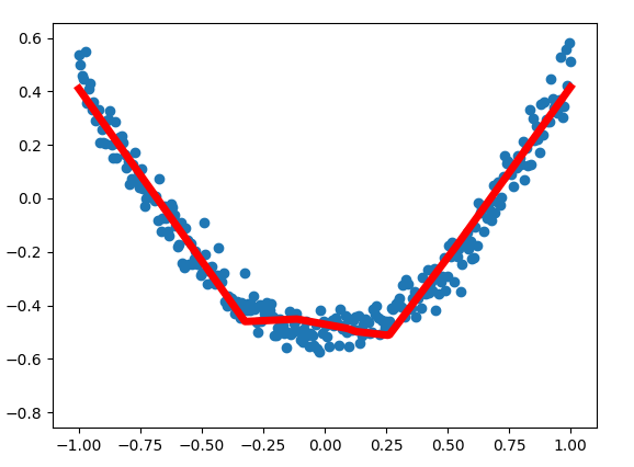
解释

程序中有两次作图，一次是散点的展示，用的函数是 ax.scatter(x_data, y_data) ，另一次是画出拟合的曲线 ax.plot(x_data, prediction_value,) ，注意，这两个函数分别对应点和线。
ax.lines.remove(lines[0]) ，你和图像的过程是逐渐向正确方向靠拢的过程，所以拟合的曲线也是动态变化的，新的曲线绘制出来的前一瞬间，需要把上一次绘制的拟合曲线删除，就是这句代买的作用
prediction_value = sess.run(prediction, feed_dict={xs: x_data}) 获取本次最新训练的预测结果
lines = ax.plot(x_data, prediction_value, 'r-', lw=5) ，将样本数据x，预测结果进行拟合，得到曲线图
plt.pause(1) ，图像暂停1s ，以供程序员观察图像

总结

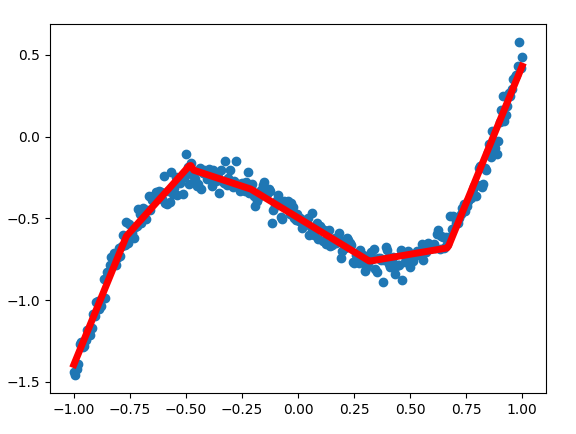
神奇的激励函数

我用这套代码拟合曲线 y_data = 2*x_data*np.square(x_data) - x_data - 0.5 + noise ，发现拟合的也不错，两个样本差别不小的。上边的图像为U行，这里为N形。如下图。

思考

这套代码差不多是我最初接触到的完整代码，但是随着看其他教程推演，第三次看这套代码才看明白。

不能说全明白，比如

问题1： 什么情况下使用什么样的激励函数 这个问题，就没有答案。
问题2：在这个demo中怎么叫训练好的模型。整个拟合过程也没有可以输出的中间参数

这个问题已经解决了

训练好的模型，就是输出中间权重参数(Weights)，和偏差参数(biases)

基本原理：上面提供的代码神经网络共三层，输入层，隐藏层，输出层，其中隐藏层和输出层使用了add_layer()函数，也就是这两层有各自的权重参数和偏差参数。因为这两层的输入(in_size)和输出(out_size)不同，所以这两层的参数的行列数(shape)也是相应不同的。

接下来我们把训练好的参数取出来

① 添加全局变量。在add_layer 函数前边添加

Weights = tf.Variable([-1,-1],dtype = tf.float32)

biases = tf.Variable([-1,-1],dtype = tf.float32)

Weights2 = tf.Variable([-1,-1],dtype = tf.float32)

biases2 = tf.Variable([-1,-1],dtype = tf.float32)

② 改返回，把

return outputs

改为

return outputs,Weights,biases

③ 改接收，把

l1 = add_layer(xs, 1, 10, activation_function=tf.nn.relu)

prediction = add_layer(l1, 10, 1, activation_function=None)

改为

l1,Weights,biases = add_layer(xs, 1, 10, activation_function=tf.nn.relu)

prediction,Weights2,biases2 = add_layer(l1, 10, 1, activation_function=None)

④ 在最后添加代码打印这些参数

print("Weights")

print(Weights)

print("biases")

print(biases)

print("Weights2")

print(Weights2)

print("biases2")

print(biases2)

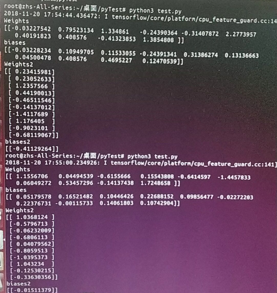
打印参数结果

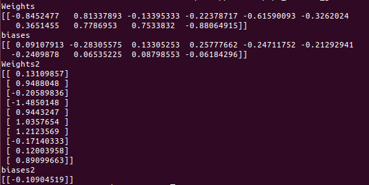
问题3：新的结果产生新的问题。在解决问题2之后，运行代码可以得到解，但是带有隐藏层和激励函数的代码每次循行之后得到的结果不同。如以上代码，去掉noise，连续运行两次，得到的是差别比较大的两组解。

之后就什么心得体会或者思考的话再想着回来补充吧