斯坦福大学卷积神经网络教程UFLDL Tutorial - Convolutional Neural Network

Convolutional Neural Network

---

Overview

A Convolutional Neural Network (CNN) is comprised of one or more convolutional layers (often with a subsampling step) and then followed by one or more fully connected layers as in a standard multilayer neural network. The architecture of a CNN is designed to take advantage of the 2D structure of an input image (or other 2D input such as a speech signal). This is achieved with local connections and tied weights followed by some form of pooling which results in translation invariant features. Another benefit of CNNs is that they are easier to train and have many fewer parameters than fully connected networks with the same number of hidden units. In this article we will discuss the architecture of a CNN and the back propagation algorithm to compute the gradient with respect to the parameters of the model in order to use gradient based optimization. See the respective tutorials on convolution andpooling for more details on those specific operations.

Architecture

A CNN consists of a number of convolutional and subsampling layers optionally followed by fully connected layers. The input to a convolutional layer is a m x m x rm x m x r image where mm is the height and width of the image and rr is the number of channels, e.g. an RGB image has r=3r=3. The convolutional layer will have kk filters (or kernels) of size n x n x qn x n x q where nn is smaller than the dimension of the image and qq can either be the same as the number of channels rr or smaller and may vary for each kernel. The size of the filters gives rise to the locally connected structure which are each convolved with the image to produce kk feature maps of size m−n+1m−n+1. Each map is then subsampled typically with mean or max pooling over p x pp x p contiguous regions where p ranges between 2 for small images (e.g. MNIST) and is usually not more than 5 for larger inputs. Either before or after the subsampling layer an additive bias and sigmoidal nonlinearity is applied to each feature map. The figure below illustrates a full layer in a CNN consisting of convolutional and subsampling sublayers. Units of the same color have tied weights.

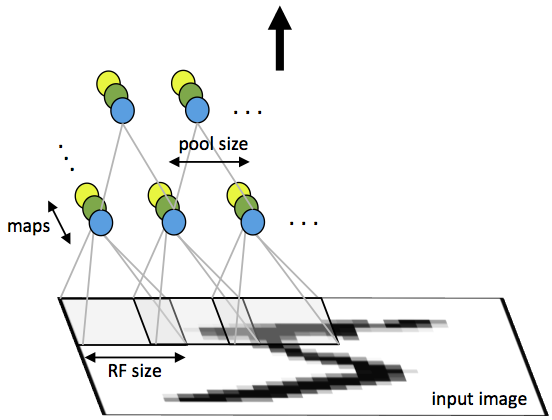
Fig 1: First layer of a convolutional neural network with pooling. Units of the same color have tied weights and units of different color represent different filter maps.

After the convolutional layers there may be any number of fully connected layers. The densely connected layers are identical to the layers in a standard multilayer neural network.

Back Propagation

Let δ(l+1)δ(l+1) be the error term for the (l+1)(l+1)-st layer in the network with a cost function J(W,b;x,y)J(W,b;x,y)where (W,b)(W,b) are the parameters and (x,y)(x,y) are the training data and label pairs. If the ll-th layer is densely connected to the (l+1)(l+1)-st layer, then the error for the ll-th layer is computed as

δ(l)=((W(l))Tδ(l+1))∙f′(z(l))δ(l)=((W(l))Tδ(l+1))∙f′(z(l))

and the gradients are

∇W(l)J(W,b;x,y)∇b(l)J(W,b;x,y)=δ(l+1)(a(l))T,=δ(l+1).∇W(l)J(W,b;x,y)=δ(l+1)(a(l))T,∇b(l)J(W,b;x,y)=δ(l+1).

If the ll-th layer is a convolutional and subsampling layer then the error is propagated through as

δ(l)k=upsample((W(l)k)Tδ(l+1)k)∙f′(z(l)k)δk(l)=upsample((Wk(l))Tδk(l+1))∙f′(zk(l))

Where kk indexes the filter number and f′(z(l)k)f′(zk(l)) is the derivative of the activation function. The upsampleoperation has to propagate the error through the pooling layer by calculating the error w.r.t to each unit incoming to the pooling layer. For example, if we have mean pooling then upsample simply uniformly distributes the error for a single pooling unit among the units which feed into it in the previous layer. In max pooling the unit which was chosen as the max receives all the error since very small changes in input would perturb the result only through that unit.

Finally, to calculate the gradient w.r.t to the filter maps, we rely on the border handling convolution operation again and flip the error matrix δ(l)kδk(l) the same way we flip the filters in the convolutional layer.

∇W(l)kJ(W,b;x,y)∇b(l)kJ(W,b;x,y)=∑i=1m(a(l)i)∗rot90(δ(l+1)k,2),=∑a,b(δ(l+1)k)a,b.∇Wk(l)J(W,b;x,y)=∑i=1m(ai(l))∗rot90(δk(l+1),2),∇bk(l)J(W,b;x,y)=∑a,b(δk(l+1))a,b.

Where a(l)a(l) is the input to the ll-th layer, and a(1)a(1) is the input image. The operation (a(l)i)∗δ(l+1)k(ai(l))∗δk(l+1) is the “valid” convolution between ii-th input in the ll-th layer and the error w.r.t. the kk-th filter.

from: http://ufldl.stanford.edu/tutorial/supervised/ConvolutionalNeuralNetwork/