Some 3D Graphics (rgl) for Classification with Splines and Logistic Regression (from The Elements of Statistical Learning)（转）

This semester I'm teaching from Hastie, Tibshirani, and Friedman's book, The Elements of Statistical Learning, 2nd Edition. The authors provide aMixture Simulation data set that has two continuous predictors and a binary outcome. This data is used to demonstrate classification procedures by plotting classification boundaries in the two predictors. For example, the figure below is a reproduction of Figure 2.5 in the book:

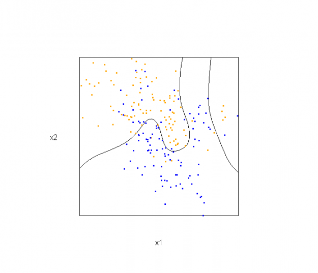
The solid line represents the Bayes decision boundary (i.e., {x: Pr("orange"|x) = 0.5}), which is computed from the model used to simulate these data. The Bayes decision boundary and other boundaries are determined by one or more surfaces (e.g., Pr("orange"|x)), which are generally omitted from the graphics. In class, we decided to use the R package rgl to create a 3D representation of this surface. Below is the code and graphic (well, a 2D projection) associated with the Bayes decision boundary:

library(rgl)
load(url("http://statweb.stanford.edu/~tibs/ElemStatLearn/datasets/ESL.mixture.rda"))
dat <- ESL.mixture

## create 3D graphic, rotate to view 2D x1/x2 projection
par3d(FOV=1,userMatrix=diag(4))
plot3d(dat$xnew[,1], dat$xnew[,2], dat$prob, type="n",
       xlab="x1", ylab="x2", zlab="",
       axes=FALSE, box=TRUE, aspect=1)

## plot points and bounding box
x1r <- range(dat$px1)
x2r <- range(dat$px2)
pts <- plot3d(dat$x[,1], dat$x[,2], 1,
              type="p", radius=0.5, add=TRUE,
              col=ifelse(dat$y, "orange", "blue"))
lns <- lines3d(x1r[c(1,2,2,1,1)], x2r[c(1,1,2,2,1)], 1)

## draw Bayes (True) decision boundary; provided by authors
dat$probm <- with(dat, matrix(prob, length(px1), length(px2)))
dat$cls <- with(dat, contourLines(px1, px2, probm, levels=0.5))
pls <- lapply(dat$cls, function(p) lines3d(p$x, p$y, z=1))

## plot marginal (w.r.t mixture) probability surface and decision plane
sfc <- surface3d(dat$px1, dat$px2, dat$prob, alpha=1.0,
            color="gray", specular="gray")
qds <- quads3d(x1r[c(1,2,2,1)], x2r[c(1,1,2,2)], 0.5, alpha=0.4,
            color="gray", lit=FALSE)

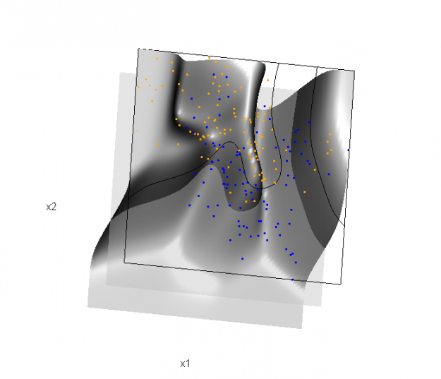
In the above graphic, the probability surface is represented in gray, and the Bayes decision boundary occurs where the plane f(x) = 0.5 (in light gray) intersects with the probability surface.

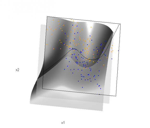
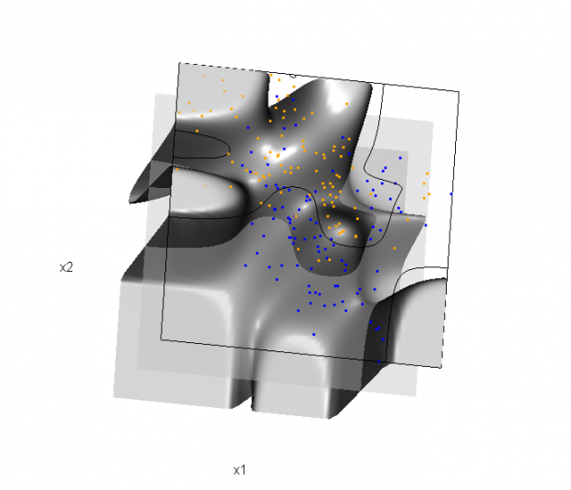
Of course, the classification task is to estimate a decision boundary given the data. Chapter 5 presents two multidimensional splines approaches, in conjunction with binary logistic regression, to estimate a decision boundary. The upper panel of Figure 5.11 in the book shows the decision boundary associated with additive natural cubic splines in x1 and x2 (4 df in each direction; 1+(4-1)+(4-1) = 7 parameters), and the lower panel shows the corresponding tensor product splines (4x4 = 16 parameters), which are much more flexible, of course. The code and graphics below reproduce the decision boundaries shown in Figure 5.11, and additionally illustrate the estimated probability surface (note: this code below should only be executed after the above code, since the 3D graphic is modified, rather than created anew):

Reproducing Figure 5.11 (top):

## clear the surface, decision plane, and decision boundary
par3d(userMatrix=diag(4)); pop3d(id=sfc); pop3d(id=qds)
for(pl in pls) pop3d(id=pl)

## fit additive natural cubic spline model
library(splines)
ddat <- data.frame(y=dat$y, x1=dat$x[,1], x2=dat$x[,2])
form.add <- y ~ ns(x1, df=3)+
                ns(x2, df=3)
fit.add  <- glm(form.add, data=ddat, family=binomial(link="logit"))

## compute probabilities, plot classification boundary
probs.add <- predict(fit.add, type="response",
                     newdata = data.frame(x1=dat$xnew[,1], x2=dat$xnew[,2]))
dat$probm.add <- with(dat, matrix(probs.add, length(px1), length(px2)))
dat$cls.add <- with(dat, contourLines(px1, px2, probm.add, levels=0.5))
pls <- lapply(dat$cls.add, function(p) lines3d(p$x, p$y, z=1))

## plot probability surface and decision plane
sfc <- surface3d(dat$px1, dat$px2, probs.add, alpha=1.0,
                 color="gray", specular="gray")
qds <- quads3d(x1r[c(1,2,2,1)], x2r[c(1,1,2,2)], 0.5, alpha=0.4,
               color="gray", lit=FALSE)

Reproducing Figure 5.11 (bottom)

## clear the surface, decision plane, and decision boundary
par3d(userMatrix=diag(4)); pop3d(id=sfc); pop3d(id=qds)
for(pl in pls) pop3d(id=pl)

## fit tensor product natural cubic spline model
form.tpr <- y ~ 0 + ns(x1, df=4, intercept=TRUE):
                    ns(x2, df=4, intercept=TRUE)
fit.tpr  <- glm(form.tpr, data=ddat, family=binomial(link="logit"))

## compute probabilities, plot classification boundary
probs.tpr <- predict(fit.tpr, type="response",
                     newdata = data.frame(x1=dat$xnew[,1], x2=dat$xnew[,2]))
dat$probm.tpr <- with(dat, matrix(probs.tpr, length(px1), length(px2)))
dat$cls.tpr <- with(dat, contourLines(px1, px2, probm.tpr, levels=0.5))
pls <- lapply(dat$cls.tpr, function(p) lines3d(p$x, p$y, z=1))

## plot probability surface and decision plane
sfc <- surface3d(dat$px1, dat$px2, probs.tpr, alpha=1.0,
                 color="gray", specular="gray")
qds <- quads3d(x1r[c(1,2,2,1)], x2r[c(1,1,2,2)], 0.5, alpha=0.4,
               color="gray", lit=FALSE)

Although the graphics above are static, it is possible to embed an interactive 3D version within a web page (e.g., see the rgl vignette; best with Google Chrome), using the rgl function writeWebGL. I gave up on trying to embed such a graphic into this WordPress blog post, but I have created a separate page for the interactive 3D version of Figure 5.11b. Duncan Murdoch's work with this package is reall nice!

This entry was posted in Technical and tagged data, graphics, programming, R, statistics on February 1, 2015.

转自：http://biostatmatt.com/archives/2659