[Scikit-learn] 1.4 Support Vector Classification

支持向量机

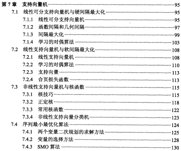
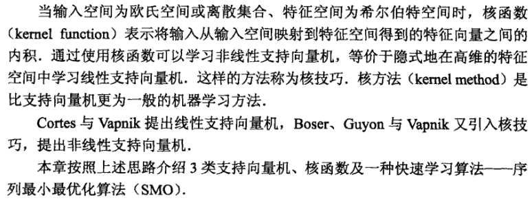
其实就是最大间隔分类器，而且是软间隔，加正则。

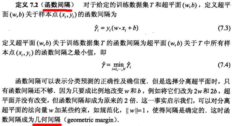
对于时间充裕的年轻人，建议SVM的原理推导一遍，过程中设计了大部分的数学优化基础，而且SVM是自成体系的sol，大有裨益。

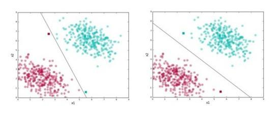
Figure, SVM试图找到右图中的“分割线”

Support vector machines (SVMs) are a set of supervised learning methods used for classification (分类), regression (回归) and outliers detection ( 异常检测).

优势

Effective in high dimensional spaces. 【高维好操作】

Still effective in cases where number of dimensions is greater than the number of samples. 【高维，例如语言模型，但效果好不好是另一码事】

Uses a subset of training points in the decision function (called support vectors), so it is also memory efficient. 【通过子集判断】

Versatile: different Kernel functions can be specified for the decision function. Common kernels are provided, but it is also possible to specify custom kernels.

劣势

If the number of features is much greater than the number of samples, the method is likely to give poor performances.

SVMs do not directly provide probability estimates, these are calculated using an expensive five-fold cross-validation.　

什么是支持向量

支持向量（support vector）：距离最接近的数据点。

间隔（margin）：支持向量定义的沿着分隔线的区域。

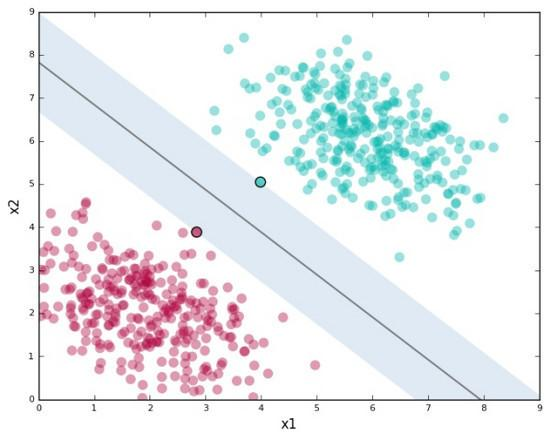
有间隔就会影响分类结果中的误差大小

SVM允许我们通过参数 C 指定愿意接受多少误差，让我们可以指定以下两者的折衷：

- 较宽的间隔。正确分类训练数据。
- C值较高，意味着训练数据上容许的误差较少

什么是核

升维使其可分

一般而言，很难找到这样的特定投影。

不过，感谢Cover定理，我们确实知道，投影到高维空间后，数据更可能线性可分。

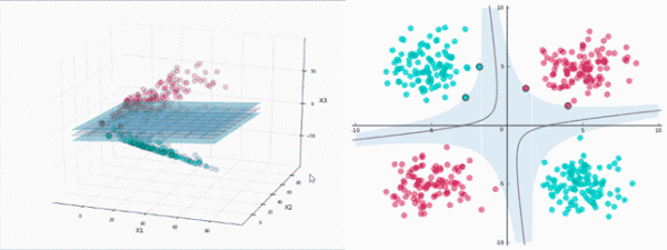
谁来做高维投影

SVM将使用一种称为核（kernels）的东西进行投影，这相当迅速。

升维且高效

需要几次运算？在二维情形下计算内积需要2次乘法、1次加法，然后平方又是1次乘法。所以总共是 4次运算，仅仅是之前先投影后计算的运算量的31% 。

看来用核函数计算所需内积要快得多。在这个例子中，这点提升可能不算什么：4次运算和13次运算。然而，如果数据点有许多维度，投影空间的维度更高，在大型数据集上，核函数节省的算力将飞速累积。这是核函数的巨大优势。

大多数SVM库内置了流行的核函数，比如多项式（Polynomial）、径向基函数（Radial Basis Function，RBF）、 Sigmoid 。当我们不进行投影时（比如本文的第一个例子），我们直接在原始空间计算点积——我们把这叫做使用线性核（linear kernel）。

径向基函数 RBF

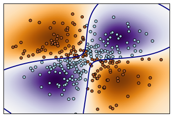
例：RBF kernel 【径向基函数 (Radial Basis Function 简称 RBF), 就是某种沿径向对称的标量函数，也是默认kernel】

"""

==============

Non-linear SVM

==============

Perform binary classification using non-linear SVC

with RBF kernel. The target to predict is a XOR of the

inputs.

The color map illustrates the decision function learned by the SVC.

"""

print(__doc__)

import numpy as np

import matplotlib.pyplot as plt

from sklearn import svm


# 生成网格型数据

xx, yy = np.meshgrid(np.linspace(-3, 3, 500), np.linspace(-3, 3, 500))

np.random.seed(0)

X = np.random.randn(300, 2)

Y = np.logical_xor(X[:, 0] > 0, X[:, 1] > 0)

# fit the model

clf = svm.NuSVC()

clf.fit(X, Y)

# plot the decision function for each datapoint on the grid

Z = clf.decision_function(np.c_[xx.ravel(), yy.ravel()])

Z = Z.reshape(xx.shape)

plt.imshow(Z, interpolation='nearest',

           extent=(xx.min(), xx.max(), yy.min(), yy.max()), aspect='auto',

           origin='lower', cmap=plt.cm.PuOr_r)

contours = plt.contour(xx, yy, Z, levels=[0], linewidths=2, linetypes='--')

plt.scatter(X[:, 0], X[:, 1], s=30, c=Y, cmap=plt.cm.Paired)

plt.xticks(())

plt.yticks(())

plt.axis([-3, 3, -3, 3])

plt.show()

变量：xx, yy

xx

Out[140]:

array([[-3.        , -2.98797595, -2.9759519 , ...,  2.9759519 ,

         2.98797595,  3.        ],

       [-3.        , -2.98797595, -2.9759519 , ...,  2.9759519 ,

         2.98797595,  3.        ],

       [-3.        , -2.98797595, -2.9759519 , ...,  2.9759519 ,

         2.98797595,  3.        ],

       ...,

       [-3.        , -2.98797595, -2.9759519 , ...,  2.9759519 ,

         2.98797595,  3.        ],

       [-3.        , -2.98797595, -2.9759519 , ...,  2.9759519 ,

         2.98797595,  3.        ],

       [-3.        , -2.98797595, -2.9759519 , ...,  2.9759519 ,

         2.98797595,  3.        ]])

yy

Out[141]:

array([[-3.        , -3.        , -3.        , ..., -3.        ,

        -3.        , -3.        ],

       [-2.98797595, -2.98797595, -2.98797595, ..., -2.98797595,

        -2.98797595, -2.98797595],

       [-2.9759519 , -2.9759519 , -2.9759519 , ..., -2.9759519 ,

        -2.9759519 , -2.9759519 ],

       ...,

       [ 2.9759519 ,  2.9759519 ,  2.9759519 , ...,  2.9759519 ,

         2.9759519 ,  2.9759519 ],

       [ 2.98797595,  2.98797595,  2.98797595, ...,  2.98797595,

         2.98797595,  2.98797595],

       [ 3.        ,  3.        ,  3.        , ...,  3.        ,

         3.        ,  3.        ]])

np.c_ 降维后的元素的reconstruct

np.c_[np.array([1,2,3]), np.array([4,5,6])]

Out[142]:

array([[1, 4],

       [2, 5],

       [3, 6]])

np.c_[np.array([[1,2,3]]), 0, 0, np.array([[4,5,6]])]

Out[143]: array([[1, 2, 3, 0, 0, 4, 5, 6]])

不同的核：Various kernels

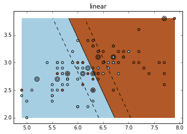
可见，RBF 的分割更为细致。

"""

================================

SVM Exercise

================================

A tutorial exercise for using different SVM kernels.

This exercise is used in the :ref:`using_kernels_tut` part of the

:ref:`supervised_learning_tut` section of the :ref:`stat_learn_tut_index`.

"""

print(__doc__)

import numpy as np

import matplotlib.pyplot as plt

from sklearn import datasets, svm

iris = datasets.load_iris()

X = iris.data

y = iris.target

X = X[y != 0, :2]

y = y[y != 0]

n_sample = len(X)

np.random.seed(0)

order = np.random.permutation(n_sample)

X = X[order]

y = y[order].astype(np.float)

# shuffle

X_train = X[:.9 * n_sample]

y_train = y[:.9 * n_sample]

X_test  = X[ .9 * n_sample:]

y_test  = y[ .9 * n_sample:]

# fit the model

for fig_num, kernel in enumerate(('linear', 'rbf', 'poly')):

    clf = svm.SVC(kernel=kernel, gamma=10)

    clf.fit(X_train, y_train)

    plt.figure(fig_num)

    plt.clf()

    plt.scatter(X[:, 0], X[:, 1], c=y, zorder=10, cmap=plt.cm.Paired)

    # Circle out the test data

    plt.scatter(X_test[:, 0], X_test[:, 1], s=80, facecolors='none', zorder=10)

    plt.axis('tight')

    x_min = X[:, 0].min()

    x_max = X[:, 0].max()

    y_min = X[:, 1].min()

    y_max = X[:, 1].max()

    XX, YY = np.mgrid[x_min:x_max:200j, y_min:y_max:200j]

    Z = clf.decision_function(np.c_[XX.ravel(), YY.ravel()])

    # Put the result into a color plot

    Z = Z.reshape(XX.shape)

    plt.pcolormesh(XX, YY, Z > 0, cmap=plt.cm.Paired)

    plt.contour(XX, YY, Z, colors=['k', 'k', 'k'], linestyles=['--', '-', '--'],

                levels=[-.5, 0, .5])

    plt.title(kernel)

plt.show()

Result:

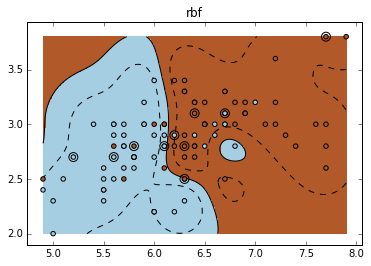
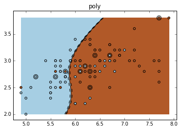
End.