
KNN笔记
KNN笔记
先简单加载一下sklearn里的数据集,然后再来讲KNN。
 import numpy as np

 import matplotlib as mpl

 import matplotlib.pyplot as plt

 from sklearn import datasets

 iris=datasets.load_iris()
看一下鸢尾花的keys:
iris.keys()
结果是:
dict_keys(['data', 'target', 'target_names', 'DESCR', 'feature_names'])
看一下文档:
print(iris.DESCR) #看看文档
文档结果:
Iris Plants Database

====================

Notes

-----

Data Set Characteristics:

    :Number of Instances: 150 (50 in each of three classes)

    :Number of Attributes: 4 numeric, predictive attributes and the class

    :Attribute Information:

        - sepal length in cm

        - sepal width in cm

        - petal length in cm

        - petal width in cm

        - class:

                - Iris-Setosa

                - Iris-Versicolour

                - Iris-Virginica

    :Summary Statistics:

    ============== ==== ==== ======= ===== ====================

                    Min  Max   Mean    SD   Class Correlation

    ============== ==== ==== ======= ===== ====================

    sepal length:   4.3  7.9   5.84   0.83    0.7826

    sepal width:    2.0  4.4   3.05   0.43   -0.4194

    petal length:   1.0  6.9   3.76   1.76    0.9490  (high!)

    petal width:    0.1  2.5   1.20  0.76     0.9565  (high!)

    ============== ==== ==== ======= ===== ====================

    :Missing Attribute Values: None

    :Class Distribution: 33.3% for each of 3 classes.

    :Creator: R.A. Fisher

    :Donor: Michael Marshall (MARSHALL%PLU@io.arc.nasa.gov)

    :Date: July, 1988

This is a copy of UCI ML iris datasets.

http://archive.ics.uci.edu/ml/datasets/Iris

The famous Iris database, first used by Sir R.A Fisher

This is perhaps the best known database to be found in the

pattern recognition literature.  Fisher's paper is a classic in the field and

is referenced frequently to this day.  (See Duda & Hart, for example.)  The

data set contains 3 classes of 50 instances each, where each class refers to a

type of iris plant.  One class is linearly separable from the other 2; the

latter are NOT linearly separable from each other.

References

----------

   - Fisher,R.A. "The use of multiple measurements in taxonomic problems"

     Annual Eugenics, 7, Part II, 179-188 (1936); also in "Contributions to

     Mathematical Statistics" (John Wiley, NY, 1950).

   - Duda,R.O., & Hart,P.E. (1973) Pattern Classification and Scene Analysis.

     (Q327.D83) John Wiley & Sons.  ISBN 0-471-22361-1.  See page 218.

   - Dasarathy, B.V. (1980) "Nosing Around the Neighborhood: A New System

     Structure and Classification Rule for Recognition in Partially Exposed

     Environments".  IEEE Transactions on Pattern Analysis and Machine

     Intelligence, Vol. PAMI-2, No. 1, 67-71.

   - Gates, G.W. (1972) "The Reduced Nearest Neighbor Rule".  IEEE Transactions

     on Information Theory, May 1972, 431-433.

   - See also: 1988 MLC Proceedings, 54-64.  Cheeseman et al"s AUTOCLASS II

     conceptual clustering system finds 3 classes in the data.

   - Many, many more ...
文档
看一下数据data:
iris.data #看看数据
数据为:
 array([[ 5.1,  3.5,  1.4,  0.2],

        [ 4.9,  3. ,  1.4,  0.2],

        [ 4.7,  3.2,  1.3,  0.2],

        [ 4.6,  3.1,  1.5,  0.2],

        [ 5. ,  3.6,  1.4,  0.2],

        [ 5.4,  3.9,  1.7,  0.4],

        [ 4.6,  3.4,  1.4,  0.3],

        [ 5. ,  3.4,  1.5,  0.2],

        [ 4.4,  2.9,  1.4,  0.2],

        [ 4.9,  3.1,  1.5,  0.1],

        [ 5.4,  3.7,  1.5,  0.2],

        [ 4.8,  3.4,  1.6,  0.2],

        [ 4.8,  3. ,  1.4,  0.1],

        [ 4.3,  3. ,  1.1,  0.1],

        [ 5.8,  4. ,  1.2,  0.2],

        [ 5.7,  4.4,  1.5,  0.4],

        [ 5.4,  3.9,  1.3,  0.4],

        [ 5.1,  3.5,  1.4,  0.3],

        [ 5.7,  3.8,  1.7,  0.3],

        [ 5.1,  3.8,  1.5,  0.3],

        [ 5.4,  3.4,  1.7,  0.2],

        [ 5.1,  3.7,  1.5,  0.4],

        [ 4.6,  3.6,  1. ,  0.2],

        [ 5.1,  3.3,  1.7,  0.5],

        [ 4.8,  3.4,  1.9,  0.2],

        [ 5. ,  3. ,  1.6,  0.2],

        [ 5. ,  3.4,  1.6,  0.4],

        [ 5.2,  3.5,  1.5,  0.2],

        [ 5.2,  3.4,  1.4,  0.2],

        [ 4.7,  3.2,  1.6,  0.2],

        [ 4.8,  3.1,  1.6,  0.2],

        [ 5.4,  3.4,  1.5,  0.4],

        [ 5.2,  4.1,  1.5,  0.1],

        [ 5.5,  4.2,  1.4,  0.2],

        [ 4.9,  3.1,  1.5,  0.1],

        [ 5. ,  3.2,  1.2,  0.2],

        [ 5.5,  3.5,  1.3,  0.2],

        [ 4.9,  3.1,  1.5,  0.1],

        [ 4.4,  3. ,  1.3,  0.2],

        [ 5.1,  3.4,  1.5,  0.2],

        [ 5. ,  3.5,  1.3,  0.3],

        [ 4.5,  2.3,  1.3,  0.3],

        [ 4.4,  3.2,  1.3,  0.2],

        [ 5. ,  3.5,  1.6,  0.6],

        [ 5.1,  3.8,  1.9,  0.4],

        [ 4.8,  3. ,  1.4,  0.3],

        [ 5.1,  3.8,  1.6,  0.2],

        [ 4.6,  3.2,  1.4,  0.2],

        [ 5.3,  3.7,  1.5,  0.2],

        [ 5. ,  3.3,  1.4,  0.2],

        [ 7. ,  3.2,  4.7,  1.4],

        [ 6.4,  3.2,  4.5,  1.5],

        [ 6.9,  3.1,  4.9,  1.5],

        [ 5.5,  2.3,  4. ,  1.3],

        [ 6.5,  2.8,  4.6,  1.5],

        [ 5.7,  2.8,  4.5,  1.3],

        [ 6.3,  3.3,  4.7,  1.6],

        [ 4.9,  2.4,  3.3,  1. ],

        [ 6.6,  2.9,  4.6,  1.3],

        [ 5.2,  2.7,  3.9,  1.4],

        [ 5. ,  2. ,  3.5,  1. ],

        [ 5.9,  3. ,  4.2,  1.5],

        [ 6. ,  2.2,  4. ,  1. ],

        [ 6.1,  2.9,  4.7,  1.4],

        [ 5.6,  2.9,  3.6,  1.3],

        [ 6.7,  3.1,  4.4,  1.4],

        [ 5.6,  3. ,  4.5,  1.5],

        [ 5.8,  2.7,  4.1,  1. ],

        [ 6.2,  2.2,  4.5,  1.5],

        [ 5.6,  2.5,  3.9,  1.1],

        [ 5.9,  3.2,  4.8,  1.8],

        [ 6.1,  2.8,  4. ,  1.3],

        [ 6.3,  2.5,  4.9,  1.5],

        [ 6.1,  2.8,  4.7,  1.2],

        [ 6.4,  2.9,  4.3,  1.3],

        [ 6.6,  3. ,  4.4,  1.4],

        [ 6.8,  2.8,  4.8,  1.4],

        [ 6.7,  3. ,  5. ,  1.7],

        [ 6. ,  2.9,  4.5,  1.5],

        [ 5.7,  2.6,  3.5,  1. ],

        [ 5.5,  2.4,  3.8,  1.1],

        [ 5.5,  2.4,  3.7,  1. ],

        [ 5.8,  2.7,  3.9,  1.2],

        [ 6. ,  2.7,  5.1,  1.6],

        [ 5.4,  3. ,  4.5,  1.5],

        [ 6. ,  3.4,  4.5,  1.6],

        [ 6.7,  3.1,  4.7,  1.5],

        [ 6.3,  2.3,  4.4,  1.3],

        [ 5.6,  3. ,  4.1,  1.3],

        [ 5.5,  2.5,  4. ,  1.3],

        [ 5.5,  2.6,  4.4,  1.2],

        [ 6.1,  3. ,  4.6,  1.4],

        [ 5.8,  2.6,  4. ,  1.2],

        [ 5. ,  2.3,  3.3,  1. ],

        [ 5.6,  2.7,  4.2,  1.3],

        [ 5.7,  3. ,  4.2,  1.2],

        [ 5.7,  2.9,  4.2,  1.3],

        [ 6.2,  2.9,  4.3,  1.3],

        [ 5.1,  2.5,  3. ,  1.1],

        [ 5.7,  2.8,  4.1,  1.3],

        [ 6.3,  3.3,  6. ,  2.5],

        [ 5.8,  2.7,  5.1,  1.9],

        [ 7.1,  3. ,  5.9,  2.1],

        [ 6.3,  2.9,  5.6,  1.8],

        [ 6.5,  3. ,  5.8,  2.2],

        [ 7.6,  3. ,  6.6,  2.1],

        [ 4.9,  2.5,  4.5,  1.7],

        [ 7.3,  2.9,  6.3,  1.8],

        [ 6.7,  2.5,  5.8,  1.8],

        [ 7.2,  3.6,  6.1,  2.5],

        [ 6.5,  3.2,  5.1,  2. ],

        [ 6.4,  2.7,  5.3,  1.9],

        [ 6.8,  3. ,  5.5,  2.1],

        [ 5.7,  2.5,  5. ,  2. ],

        [ 5.8,  2.8,  5.1,  2.4],

        [ 6.4,  3.2,  5.3,  2.3],

        [ 6.5,  3. ,  5.5,  1.8],

        [ 7.7,  3.8,  6.7,  2.2],

        [ 7.7,  2.6,  6.9,  2.3],

        [ 6. ,  2.2,  5. ,  1.5],

        [ 6.9,  3.2,  5.7,  2.3],

        [ 5.6,  2.8,  4.9,  2. ],

        [ 7.7,  2.8,  6.7,  2. ],

        [ 6.3,  2.7,  4.9,  1.8],

        [ 6.7,  3.3,  5.7,  2.1],

        [ 7.2,  3.2,  6. ,  1.8],

        [ 6.2,  2.8,  4.8,  1.8],

        [ 6.1,  3. ,  4.9,  1.8],

        [ 6.4,  2.8,  5.6,  2.1],

        [ 7.2,  3. ,  5.8,  1.6],

        [ 7.4,  2.8,  6.1,  1.9],

        [ 7.9,  3.8,  6.4,  2. ],

        [ 6.4,  2.8,  5.6,  2.2],

        [ 6.3,  2.8,  5.1,  1.5],

        [ 6.1,  2.6,  5.6,  1.4],

        [ 7.7,  3. ,  6.1,  2.3],

        [ 6.3,  3.4,  5.6,  2.4],

        [ 6.4,  3.1,  5.5,  1.8],

        [ 6. ,  3. ,  4.8,  1.8],

        [ 6.9,  3.1,  5.4,  2.1],

        [ 6.7,  3.1,  5.6,  2.4],

        [ 6.9,  3.1,  5.1,  2.3],

        [ 5.8,  2.7,  5.1,  1.9],

        [ 6.8,  3.2,  5.9,  2.3],

        [ 6.7,  3.3,  5.7,  2.5],

        [ 6.7,  3. ,  5.2,  2.3],

        [ 6.3,  2.5,  5. ,  1.9],

        [ 6.5,  3. ,  5.2,  2. ],

        [ 6.2,  3.4,  5.4,  2.3],

        [ 5.9,  3. ,  5.1,  1.8]])
数据data
可见data为150行,每行4列的数据。
看一下target:
iris.target #看看对应的目标值
target结果为:
array([0, 0, 0, 0, 0, 0, 0, 0, 0, 0, 0, 0, 0, 0, 0, 0, 0, 0, 0, 0, 0, 0, 0,

       0, 0, 0, 0, 0, 0, 0, 0, 0, 0, 0, 0, 0, 0, 0, 0, 0, 0, 0, 0, 0, 0, 0,

       0, 0, 0, 0, 1, 1, 1, 1, 1, 1, 1, 1, 1, 1, 1, 1, 1, 1, 1, 1, 1, 1, 1,

       1, 1, 1, 1, 1, 1, 1, 1, 1, 1, 1, 1, 1, 1, 1, 1, 1, 1, 1, 1, 1, 1, 1,

       1, 1, 1, 1, 1, 1, 1, 1, 2, 2, 2, 2, 2, 2, 2, 2, 2, 2, 2, 2, 2, 2, 2,

       2, 2, 2, 2, 2, 2, 2, 2, 2, 2, 2, 2, 2, 2, 2, 2, 2, 2, 2, 2, 2, 2, 2,

       2, 2, 2, 2, 2, 2, 2, 2, 2, 2, 2, 2])
看一下target_names:
iris.target_names #看看目标值对应的目标名称
arget_names结果为:
array(['setosa', 'versicolor', 'virginica'],

      dtype='<U10')
也就是target的0,1,2分别对应的鸢尾花的名称就是这三个。
看一下4列数据(也就是data)分别是指什么
iris.feature_names #看看四个数据对应的是什么
可以看到结果为:
['sepal length (cm)',

 'sepal width (cm)',

 'petal length (cm)',

 'petal width (cm)']
也就是4列数据分别代表花萼的长,花萼的宽,花瓣的长,花瓣的宽。
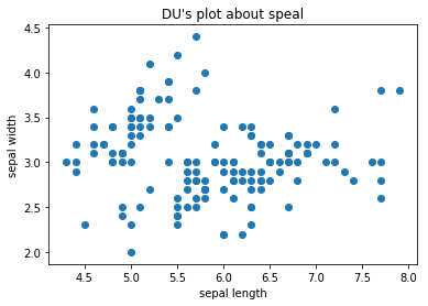
看一下花萼的数据,也就是前两列的数据:
 #看一下花萼的散点图

 X=iris.data[:,:2]

 plt.scatter(X[:,0],X[:,1])

 plt.xlabel("sepal length")

 plt.ylabel("sepal width")

 plt.title("DU's plot about speal")

 plt.show()
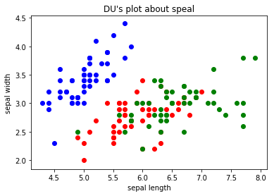
把三种花的散点图区分一下:
 #把三种花的花萼的散点图画出来

 y=iris.target

 plt.scatter(X[y==0,0],X[y==0,1],color='b')

 plt.scatter(X[y==1,0],X[y==1,1],color='r')

 plt.scatter(X[y==2,0],X[y==2,1],color='g')

 plt.xlabel("sepal length")

 plt.ylabel("sepal width")

 plt.title("DU's plot about speal")

 plt.show()
再看一下花瓣的散点图:
 Petal=iris.data[:,2:]

 y=iris.target

 plt.scatter(Petal[y==0,0],Petal[y==0,1],color='b')

 plt.scatter(Petal[y==1,0],Petal[y==1,1],color='r')

 plt.scatter(Petal[y==2,0],Petal[y==2,1],color='g')

 plt.xlabel("Petal length")

 plt.ylabel("Petal width")

 plt.title("DU's plot about Petal")

 plt.show()
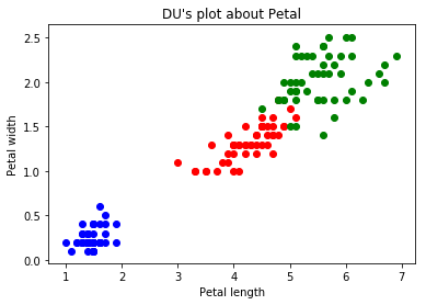
看到花瓣的散点图,那么就说一下KNN,那现在假设,花瓣散点图里来了一个长度为2cm,宽度主0.5cm的一个点,那么这个点代表的是哪个鸢尾呢?一般的人就能推出这个点应该是跟蓝色点是一类的,因为新进来的点是离蓝色的区域最近的,而离其他的红色或者绿色区域都很远。那么,这就是KNN的一个思想了。
比如现假设有如下场景,模拟有如下数据:
 raw_X=[[1,2],

        [2.8,2.5],

        [4,3.2],

        [2,1.5],

        [6,7.8],

        [8,5],

        [9,7],

        [7,8.5],

        [10,9.7],

       ]

 raw_y=[0,0,0,0,1,1,1,1,1]

 X_train=np.array(raw_X)

 y_train=np.array(raw_y)
现在有一个数据x(设置为绿色的点)进来了,要判断这个数据是属于哪一类的:
 x=np.array([7.5,6.5])

 plt.scatter(X_train[y_train==0,0],X_train[y_train==0,1])

 plt.scatter(X_train[y_train==1,0],X_train[y_train==1,1],color='r')

 plt.scatter(x[0],x[1],color='g')

 plt.show()
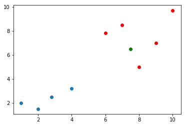
那么,按照KNN的思路就需求,求出这个里面,所有点离这个绿色点的距离了,看这个绿色的点离哪些是最近的。
那么,根据欧拉距离,一般程序员就可以写出这样的代码了:
 from math import sqrt

 distances=[]

 for x_train in X_train:

     d=sqrt(np.sum(x_train-x)**2)

     distances.append(d)
当然,根据欧拉距离,不一般的程序员是会这么写:
distances=[sqrt(np.sum(x_train-x)**2) for x_train in X_train]
而结果distances都会是:
[11.0, 8.7, 6.8, 10.5, 0.20000000000000018, 1.0, 2.0, 1.5, 5.699999999999999]
接着,算出距离最近元素的索引,进而拿到距离最近的值:
 nearest=np.argsort(distances)

 topK_y=[y_train[i] for neighbor in nearest[:5]]

 from collections import Counter

 votes=Counter(topK_y)

 predict_y=votes.most_common(1)[0][0]

 predict_y
结果明显是1。
KNN笔记的更多相关文章
- 机器学习实战笔记(Python实现)-01-K近邻算法(KNN)
--------------------------------------------------------------------------------------- 本系列文章为<机器 ...
- 第2章KNN算法笔记_函数classify0
<机器学习实战>知识点笔记目录 K-近邻算法(KNN)思想: 1,计算未知样本与所有已知样本的距离 2,按照距离递增排序,选前K个样本(K<20) 3,针对K个样本统计各个分类的出现 ...
- opencv2.4.13+python2.7学习笔记--使用 knn对手写数字OCR
阅读对象:熟悉knn.了解opencv和python. 1.knn理论介绍:算法学习笔记:knn理论介绍 2. opencv中knn函数 路径:opencv\sources\modules\ml\in ...
- 机器学习笔记(5) KNN算法
这篇其实应该作为机器学习的第一篇笔记的,但是在刚开始学习的时候,我还没有用博客记录笔记的打算.所以也就想到哪写到哪了. 你在网上搜索机器学习系列文章的话,大部分都是以KNN(k nearest nei ...
- 学习笔记之k-nearest neighbors algorithm (k-NN)
k-nearest neighbors algorithm - Wikipedia https://en.wikipedia.org/wiki/K-nearest_neighbors_algorith ...
- 机器学习实战(Machine Learning in Action)学习笔记————02.k-邻近算法(KNN)
机器学习实战(Machine Learning in Action)学习笔记————02.k-邻近算法(KNN) 关键字:邻近算法(kNN: k Nearest Neighbors).python.源 ...
- kNN算法笔记
kNN算法笔记 标签(空格分隔): 机器学习 kNN是什么 kNN算法是k-NearestNeighbor算法,也就是k邻近算法.是监督学习的一种.所谓监督学习就是有训练数据,训练数据有label标好 ...
- retrival and clustering: week 2 knn & LSH 笔记
华盛顿大学 <机器学习> 笔记. knn k-nearest-neighbors : k近邻法 给定一个 数据集,对于查询的实例,在数据集中找到与这个实例最邻近的k个实例,然后再根据k个最 ...
- 【cs231n作业笔记】一:KNN分类器
安装anaconda,下载assignment作业代码 作业代码数据集等2018版基于python3.6 下载提取码4put 本课程内容参考: cs231n官方笔记地址 贺完结!CS231n官方笔记授 ...
随机推荐
- [持续更新]Python 笔记
本文以 Python 2.7 为基础. lambda 函数实现递归 方法一:传递一个 self 参数 求阶乘: frac = lambda self, x: self(self, x - 1) * x ...
- stm32寄存器版学习笔记04 定时计数器中断
STM32共有8个定时计数器,其中TIME1和TIME8是高级定时器,TIME2~TIME5是通用定时器,TIME6和TIME7是基本定时器.以TIME3为例总结定时计数器的基本用法. 1.TIM3的 ...
- 项目文件中的已知 NuGet 属性(使用这些属性,创建 NuGet 包就可以不需要 nuspec 文件啦)
知道了 csproj 文件中的一些常用 NuGet 属性,创建 NuGet 包时就可以充分发挥新 Sdk 自动生成 NuGet 包的优势,不需要 nuspec 文件啦.(毕竟 nuspec 文件没有 ...
- Git与github常用命令
Git项目与github建立联系 首先,需要在github上建立一个repository mkdir github-project cd github-project git init 此时githu ...
- arangodb 安装简单试用
备注: 测试环境使用的是docker 1. 安装 docker run -p 8529:8529 -e ARANGO_ROOT_PASSWORD=openSesame arangodb/aran ...
- CentOS6.5安装Cacti统计图乱码解决
原创作品,允许转载,转载时请务必以超链接形式标明文章 原始出处 .作者信息和本声明.否则将追究法律责任.http://fengwan.blog.51cto.com/508652/1430505 这个就 ...
- c/c++中system函数在Linux和windows下区别
windows 在windows下的system函数中命令可以不区别大小写! 功 能: 发出一个DOS命令 #include <stdlib.h> int system(char *com ...
- CMake尝鲜
安装gcc,cmake,g++,gdb sudo apt-get install gcc cmake g++ gdb sudo apt-get update && sudo apt-g ...
- Linux make menuconfig报错 Your display is too small to run Menuconfig!
在没有全屏的状态下执行 make menuconfig,如果报下面的错误,表示终端的窗口太小,需要放大窗口或者全屏操作. ## using defaults found in /dev/null#Yo ...
- Linux 根文件系统目录结构
/:根目录 /bin:linux的常用命令 /sbin:linux的常用命令 /lib:库文件(so.elf) /etc:系统配置文件和脚本文件 /sys:驱动相关的信息 /dev:设备节点目录 /p ...