吴恩达课后作业学习2-week3-tensorflow learning-1-例子学习

参考：https://blog.csdn.net/u013733326/article/details/79971488

使用TensorFlow构建你的第一个神经网络

我们将会使用TensorFlow构建一个神经网络，需要记住的是实现模型需要做以下两个步骤： 
1. 创建计算图 
2. 运行计算图

该神经网络的目标是：判断图片表示的是什么数字（0-5）

• 训练集：有从0到5的数字的1080张图片(64x64像素)，每个数字拥有180张图片。
• 测试集：有从0到5的数字的120张图片(64x64像素)，每个数字拥有5张图片。

建立的模型是：LINEAR -> RELU -> LINEAR -> RELU -> LINEAR -> SOFTMAX，SIGMOID输出层已经转换为SOFTMAX。

当有两个以上的类时，一个SOFTMAX层将SIGMOID一般化，SIGMOID一般用于二分类中

这是一个三层神经网络

1.加载数据

X_train_orig , Y_train_orig , X_test_orig , Y_test_orig , classes = tf_utils.load_dataset()

随机查看加载的数据：

index =
plt.imshow(X_train_orig[index])
print("Y = " + str(np.squeeze(Y_train_orig[:,index])))

返回：

Y = 

图示：

index =
plt.imshow(X_train_orig[index])
print("Y = " + str(np.squeeze(Y_train_orig[:,index])))

返回：

Y = 

图示：

2.处理数据

1.首先将数据集进行扁平化

2.除以255进行归一化，将像素值由（0，255）变为（0，1）

3.并将标签Y转成独热编码

X_train_flatten = X_train_orig.reshape(X_train_orig.shape[],-).T #每一列就是一个样本
X_test_flatten = X_test_orig.reshape(X_test_orig.shape[],-).T

#归一化数据
X_train = X_train_flatten /
X_test = X_test_flatten / 

#转换为独热矩阵
Y_train = tf_utils.convert_to_one_hot(Y_train_orig,)
Y_test = tf_utils.convert_to_one_hot(Y_test_orig,)

print("训练集样本数 = " + str(X_train.shape[]))
print("测试集样本数 = " + str(X_test.shape[]))
print("X_train.shape: " + str(X_train.shape))
print("Y_train.shape: " + str(Y_train.shape))
print("X_test.shape: " + str(X_test.shape))
print("Y_test.shape: " + str(Y_test.shape))

返回：

训练集样本数 =
测试集样本数 =
X_train.shape: (, )
Y_train.shape: (, )
X_test.shape: (, )
Y_test.shape: (, )

3.创建占位符 —— X，Y

这将允许我们稍后在运行会话时传递您的训练数据

def create_placeholders(n_x,n_y):
    """
    为TensorFlow会话创建占位符
    参数：
        n_x - 一个实数，图片向量的大小（** = ）
        n_y - 一个实数，分类数（从0到5，所以n_y = ）

    返回：
        X - 一个数据输入的占位符，维度为[n_x, None]，dtype = "float"
        Y - 一个对应输入的标签的占位符，维度为[n_Y,None]，dtype = "float"

    提示：
        使用None，因为它让我们可以灵活处理占位符提供的样本数量。事实上，测试/训练期间的样本数量是不同的。

    """

    X = tf.placeholder(tf.float32, [n_x, None], name="X")
    Y = tf.placeholder(tf.float32, [n_y, None], name="Y")

    return X, Y

测试：

X, Y = create_placeholders(, )
print("X = " + str(X))
print("Y = " + str(Y))

返回：

X = Tensor("X_2:0", shape=(, ?), dtype=float32)
Y = Tensor("Y:0", shape=(, ?), dtype=float32)

4.初始化参数

使用Xavier初始化权重w和用零来初始化偏差b,即：

W1 = tf.get_variable("W1", [,], initializer = tf.contrib.layers.xavier_initializer(seed = ))
b1 = tf.get_variable("b1", [,], initializer = tf.zeros_initializer())

⚠️这里使用get_variable()函数的原因：

tf.Variable() 每次都在创建新对象，对于get_variable()来说，对于已经创建的变量对象，就把那个对象返回，如果没有创建变量对象的话，就创建一个新的。

def initialize_parameters():
    """
    初始化神经网络的参数，参数的维度如下：
        W1 : [, ]
        b1 : [, ]
        W2 : [, ]
        b2 : [, ]
        W3 : [, ]
        b3 : [, ]

    返回：
        parameters - 包含了W和b的字典

    """

    tf.set_random_seed() #指定随机种子

    W1 = tf.get_variable("W1",[,],initializer=tf.contrib.layers.xavier_initializer(seed=))
    b1 = tf.get_variable("b1",[,],initializer=tf.zeros_initializer())
    W2 = tf.get_variable("W2", [, ], initializer = tf.contrib.layers.xavier_initializer(seed=))
    b2 = tf.get_variable("b2", [, ], initializer = tf.zeros_initializer())
    W3 = tf.get_variable("W3", [, ], initializer = tf.contrib.layers.xavier_initializer(seed=))
    b3 = tf.get_variable("b3", [, ], initializer = tf.zeros_initializer())

    parameters = {"W1": W1,
                  "b1": b1,
                  "W2": W2,
                  "b2": b2,
                  "W3": W3,
                  "b3": b3}

    return parameters

测试：

tf.reset_default_graph() #用于清除默认图形堆栈并重置全局默认图形。 

with tf.Session() as sess:
    parameters = initialize_parameters()
    print("W1 = " + str(parameters["W1"]))
    print("b1 = " + str(parameters["b1"]))
    print("W2 = " + str(parameters["W2"]))
    print("b2 = " + str(parameters["b2"]))
    print("W3 = " + str(parameters["W3"]))
    print("b3 = " + str(parameters["b3"]))

返回：

W1 = <tf.Variable 'W1:0' shape=(, ) dtype=float32_ref>
b1 = <tf.Variable 'b1:0' shape=(, ) dtype=float32_ref>
W2 = <tf.Variable 'W2:0' shape=(, ) dtype=float32_ref>
b2 = <tf.Variable 'b2:0' shape=(, ) dtype=float32_ref>
W3 = <tf.Variable 'W3:0' shape=(, ) dtype=float32_ref>
b3 = <tf.Variable 'b3:0' shape=(, ) dtype=float32_ref>

正如预期的那样，这些参数只有物理空间，但是还没有被赋值，这是因为没有通过session执行。

5.前向传播

在TensorFlow中实现前向传播，该函数将接受一个字典参数并完成前向传播，它会用到以下代码：

• tf.add(…) ：加法
• tf.matmul(… , …) ：矩阵乘法
• tf.nn.relu(…) ：Relu激活函数

我们要实现神经网络的前向传播，我们会拿numpy与TensorFlow实现的神经网络的代码作比较。最重要的是前向传播要在Z3处停止，因为在TensorFlow中最后的线性输出层的输出作为计算损失函数的输入，所以不需要A3.

def forward_propagation(X,parameters):
    """
    实现一个模型的前向传播，模型结构为LINEAR -> RELU -> LINEAR -> RELU -> LINEAR -> SOFTMAX

    参数：
        X - 输入数据的占位符，维度为（输入节点数量，样本数量）
        parameters - 包含了W和b的参数的字典

    返回：
        Z3 - 最后一个LINEAR节点的输出

    """

    W1 = parameters['W1']
    b1 = parameters['b1']
    W2 = parameters['W2']
    b2 = parameters['b2']
    W3 = parameters['W3']
    b3 = parameters['b3']

    Z1 = tf.add(tf.matmul(W1,X),b1)        # Z1 = np.dot(W1, X) + b1
    #Z1 = tf.matmul(W1,X) + b1             #也可以这样写
    A1 = tf.nn.relu(Z1)                    # A1 = relu(Z1)
    Z2 = tf.add(tf.matmul(W2, A1), b2)     # Z2 = np.dot(W2, a1) + b2
    A2 = tf.nn.relu(Z2)                    # A2 = relu(Z2)
    Z3 = tf.add(tf.matmul(W3, A2), b3)     # Z3 = np.dot(W3,Z2) + b3

    return Z3

测试：

tf.reset_default_graph() #用于清除默认图形堆栈并重置全局默认图形。
with tf.Session() as sess:
    X,Y = create_placeholders(,)
    parameters = initialize_parameters()
    Z3 = forward_propagation(X,parameters)
    print("Z3 = " + str(Z3))

返回：

Z3 = Tensor("Add_2:0", shape=(, ?), dtype=float32)

可见到这里还是不能够确定传入的mini_batch_size的大小，所以是问号？

前向传播不会输出任何cache，当我们完成反向传播的时候你就会明白了

6.计算成本

tf.reduce_mean(tf.nn.softmax_cross_entropy_with_logits(logits = ..., labels = ...))

函数为：

def compute_cost(Z3,Y):
    """
    计算成本

    参数：
        Z3 - 前向传播的结果
        Y - 标签，一个占位符，和Z3的维度相同

    返回：
        cost - 成本值

    """
    logits = tf.transpose(Z3) #转置
    labels = tf.transpose(Y)  #转置

    cost = tf.reduce_mean(tf.nn.softmax_cross_entropy_with_logits(logits=logits,labels=labels))

    return cost

测试：

tf.reset_default_graph()

with tf.Session() as sess:
    X,Y = create_placeholders(,)
    parameters = initialize_parameters()
    Z3 = forward_propagation(X,parameters)
    cost = compute_cost(Z3,Y)
    print("cost = " + str(cost))

返回：

cost = Tensor("Mean:0", shape=(), dtype=float32)

这里有个警告：

WARNING:tensorflow:From <ipython-input--fa19d65a87cf>:: softmax_cross_entropy_with_logits (from tensorflow.python.ops.nn_ops) is deprecated and will be removed in a future version.
Instructions for updating:

Future major versions of TensorFlow will allow gradients to flow
into the labels input on backprop by default.

See `tf.nn.softmax_cross_entropy_with_logits_v2`.

其实就是应该使用新的成本计算函数tf.nn.softmax_cross_entropy_with_logits_v2

改后：

def compute_cost(Z3,Y):
    """
    计算成本

    参数：
        Z3 - 前向传播的结果
        Y - 标签，一个占位符，和Z3的维度相同

    返回：
        cost - 成本值

    """
    logits = tf.transpose(Z3) #转置
    labels = tf.transpose(Y)  #转置

    cost = tf.reduce_mean(tf.nn.softmax_cross_entropy_with_logits_v2(logits=logits,labels=labels))

    return cost

7.反向传播和更新参数

得益于编程框架，所有反向传播和参数更新都在1行代码中处理。

计算成本函数后，将创建一个“optimizer”对象，定义使用的优化算法和学习率等参数。

运行tf.session时，必须将此对象与成本函数一起调用，当被调用时，它将使用所选择的方法和学习速率对给定成本进行优化。

比如下面使用的是梯度下降法GD对成本进行优化：

optimizer = tf.train.GradientDescentOptimizer(learning_rate = learning_rate).minimize(cost)

要进行优化，应该这样做：

_ , c = sess.run([optimizer,cost],feed_dict={X:mini_batch_X,Y:mini_batch_Y})

feed_dict为占位符传入参数，其实就是指定一次迭代训练/测试的照片的数量

编写代码时，我们经常使用 _ 作为一次性变量来存储我们稍后不需要使用的值。 这里，_具有我们不需要的优化器的评估值（并且c取值为成本变量的值）

8.整合函数，建立模型

def model(X_train,Y_train,X_test,Y_test,
        learning_rate=0.0001,num_epochs=,minibatch_size=,
        print_cost=True,is_plot=True):
    """
    实现一个三层的TensorFlow神经网络：LINEAR->RELU->LINEAR->RELU->LINEAR->SOFTMAX

    参数：
        X_train - 训练集，维度为（输入大小（输入节点数量） = , 样本数量 = ）
        Y_train - 训练集分类数量，维度为（输出大小(输出节点数量) = , 样本数量 = ）
        X_test - 测试集，维度为（输入大小（输入节点数量） = , 样本数量 = ）
        Y_test - 测试集分类数量，维度为（输出大小(输出节点数量) = , 样本数量 = ）
        learning_rate - 学习速率
        num_epochs - 整个训练集的遍历次数
        mini_batch_size - 每个小批量数据集的大小
        print_cost - 是否打印成本，每100代打印一次
        is_plot - 是否绘制曲线图

    返回：
        parameters - 学习后的参数

    """
    ops.reset_default_graph()                #能够重新运行模型而不覆盖tf变量
    tf.set_random_seed()
    seed =
    (n_x , m)  = X_train.shape               #获取输入节点数量和样本数
    n_y = Y_train.shape[]                   #获取输出节点数量
    costs = []                               #成本集

    #给X和Y创建placeholder
    X,Y = create_placeholders(n_x,n_y)

    #初始化参数
    parameters = initialize_parameters()

    #前向传播
    Z3 = forward_propagation(X,parameters)

    #计算成本
    cost = compute_cost(Z3,Y)

    #反向传播，使用Adam优化
    optimizer = tf.train.AdamOptimizer(learning_rate=learning_rate).minimize(cost)

    #初始化所有的变量
    init = tf.global_variables_initializer()

    #开始会话并计算
    with tf.Session() as sess:
        #初始化
        sess.run(init)

        #正常训练的循环
        for epoch in range(num_epochs):

            epoch_cost =   #每代的成本
            num_minibatches = int(m / minibatch_size)    #minibatch的总数量
            seed = seed +
            #打乱来为数据分批，seed的作用是保证我们打乱后的数据和作者的相同
            minibatches = tf_utils.random_mini_batches(X_train,Y_train,minibatch_size,seed)

            for minibatch in minibatches:

                #选择一个minibatch
                (minibatch_X,minibatch_Y) = minibatch

                #数据已经准备好了，开始运行session
                _ , minibatch_cost = sess.run([optimizer,cost],feed_dict={X:minibatch_X,Y:minibatch_Y})

                #计算这个minibatch在这一代中所占的误差
                epoch_cost = epoch_cost + minibatch_cost / num_minibatches

            #记录并打印成本
            ## 记录成本
            if epoch %  == :
                costs.append(epoch_cost)
                #是否打印：
                if print_cost and epoch %  == :
                        print("epoch = " + str(epoch) + "    epoch_cost = " + str(epoch_cost))

        #是否绘制图谱
        if is_plot:
            plt.plot(np.squeeze(costs))
            plt.ylabel('cost')
            plt.xlabel('iterations (per tens)')
            plt.title("Learning rate =" + str(learning_rate))
            plt.show()

        #保存学习后的参数
        parameters = sess.run(parameters)
        print("参数已经保存到session。")

        #计算当前的预测结果
        correct_prediction = tf.equal(tf.argmax(Z3),tf.argmax(Y))

        #计算准确率
        accuracy = tf.reduce_mean(tf.cast(correct_prediction,"float"))

        print("训练集的准确率：", accuracy.eval({X: X_train, Y: Y_train}))
        print("测试集的准确率:", accuracy.eval({X: X_test, Y: Y_test}))

        return parameters

我们来正式运行一下模型，请注意，这次的运行时间大约在5-8分钟左右，如果在epoch = 100的时候，你的epoch_cost = 1.01645776539的值和我相差过大，那么你就立即停止，回头检查一下哪里出了问题。

测试：

#开始时间
start_time = time.clock()
#开始训练
parameters = model(X_train, Y_train, X_test, Y_test)
#结束时间
end_time = time.clock()
#计算时差
print("CPU的执行时间 = " + str(end_time - start_time) + " 秒" )

在jupyter运行的过程中，遇见错误：

OMP: Error #: Initializing libiomp5.dylib, but found libiomp5.dylib already initialized.
OMP: Hint This means that multiple copies of the OpenMP runtime have been linked into the program. That is dangerous, since it can degrade performance or cause incorrect results. The best thing to do is to ensure that only a single OpenMP runtime is linked into the process, e.g. by avoiding static linking of the OpenMP runtime in any library. As an unsafe, unsupported, undocumented workaround you can set the environment variable KMP_DUPLICATE_LIB_OK=TRUE to allow the program to continue to execute, but that may cause crashes or silently produce incorrect results. For more information, please see http://www.intel.com/software/products/support/.
[I ::17.486 NotebookApp] KernelRestarter: restarting kernel (/), keep random ports
kernel eb597a64-a8c0-49e5-82f2-a853f6c8b72a restarted

导致重启，一直不能成功跑完，解决办法是在运行之前先运行：

import os
os.environ["KMP_DUPLICATE_LIB_OK"]="TRUE"

如果你没有解决，更多的解决办法可见：https://github.com/dmlc/xgboost/issues/1715

返回：

epoch =     epoch_cost = 1.8557019125331538
epoch =     epoch_cost = 1.0172552520578557
epoch =     epoch_cost = 0.7331836395191423
epoch =     epoch_cost = 0.5730706308827257
epoch =     epoch_cost = 0.46857346774953773
epoch =     epoch_cost = 0.38122756237333466
epoch =     epoch_cost = 0.313796519781604
epoch =     epoch_cost = 0.2537061707539992
epoch =     epoch_cost = 0.20388749196673892
epoch =     epoch_cost = 0.16644730599540652
epoch =     epoch_cost = 0.1466932777654041
epoch =     epoch_cost = 0.10728540858536052
epoch =     epoch_cost = 0.08660263003724997
epoch =     epoch_cost = 0.05934071975449723
epoch =     epoch_cost = 0.052284905574086944

参数已经保存到session。
训练集的准确率： 0.9990741
测试集的准确率: 0.725
CPU的执行时间 = 1185.838935 秒

图示：

现在，我们的算法已经可以识别0-5的手势符号了，准确率在72.5%。
  我们的模型看起来足够大了，可以适应训练集，但是考虑到训练与测试的差异，你也完全可以尝试添加L2或者dropout来减少过拟合。将session视为一组代码来训练模型，在每个minibatch上运行会话时，都会训练我们的参数，总的来说，你已经运行了很多次（1500代），直到你获得训练有素的参数。

9.使用训练好的模型来测试

使用保存在session中训练好的参数值parameters

import matplotlib.pyplot as plt # plt 用于显示图片
import matplotlib.image as mpimg # mpimg 用于读取图片
import numpy as np

#这是博主自己拍的图片
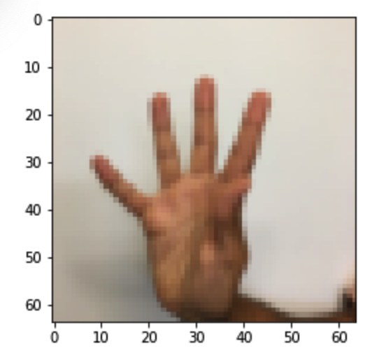
my_image1 = "5.png"                                            #定义图片名称
fileName1 = "./datasets/fingers/" + my_image1                      #图片地址
image1 = mpimg.imread(fileName1)                               #读取图片
plt.imshow(image1)                                             #显示图片
my_image1 = image1.reshape(, *  * ).T                    #重构图片
my_image_prediction = tf_utils.predict(my_image1, parameters)  #开始预测
print("预测结果: y = " + str(np.squeeze(my_image_prediction)))

返回：

预测结果: y = 

图示：

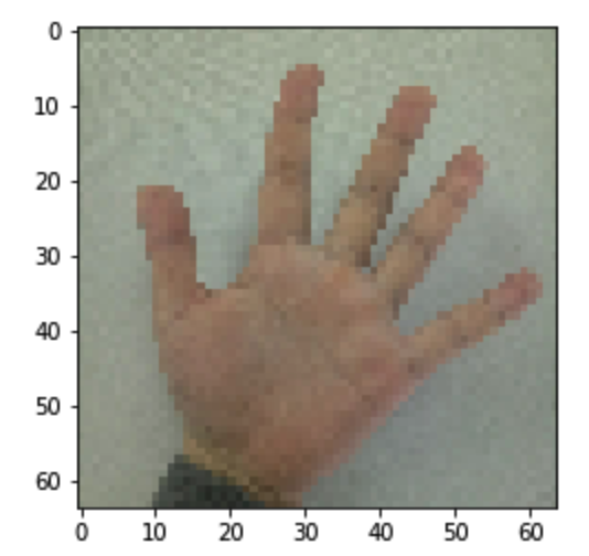
my_image1 = "4.png"                                            #定义图片名称
fileName1 = "./datasets/fingers/" + my_image1                      #图片地址
image1 = mpimg.imread(fileName1)                               #读取图片
plt.imshow(image1)                                             #显示图片
my_image1 = image1.reshape(, *  * ).T                    #重构图片
my_image_prediction = tf_utils.predict(my_image1, parameters)  #开始预测
print("预测结果: y = " + str(np.squeeze(my_image_prediction)))

返回：

预测结果: y = 

图示：

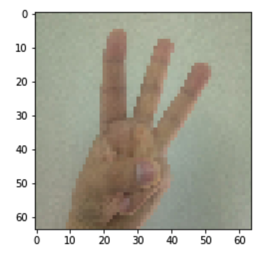
my_image1 = "3.png"                                            #定义图片名称
fileName1 = "./datasets/fingers/" + my_image1                      #图片地址
image1 = mpimg.imread(fileName1)                               #读取图片
plt.imshow(image1)                                             #显示图片
my_image1 = image1.reshape(, *  * ).T                    #重构图片
my_image_prediction = tf_utils.predict(my_image1, parameters)  #开始预测
print("预测结果: y = " + str(np.squeeze(my_image_prediction)))

返回：

预测结果: y = 

图示：

my_image1 = "2.png"                                            #定义图片名称
fileName1 = "./datasets/fingers/" + my_image1                      #图片地址
image1 = mpimg.imread(fileName1)                               #读取图片
plt.imshow(image1)                                             #显示图片
my_image1 = image1.reshape(, *  * ).T                    #重构图片
my_image_prediction = tf_utils.predict(my_image1, parameters)  #开始预测
print("预测结果: y = " + str(np.squeeze(my_image_prediction)))

返回：

预测结果: y = 

图示：

my_image1 = "1.png"                                            #定义图片名称
fileName1 = "./datasets/fingers/" + my_image1                      #图片地址
image1 = mpimg.imread(fileName1)                               #读取图片
plt.imshow(image1)                                             #显示图片
my_image1 = image1.reshape(, *  * ).T                    #重构图片
my_image_prediction = tf_utils.predict(my_image1, parameters)  #开始预测
print("预测结果: y = " + str(np.squeeze(my_image_prediction)))

返回：

预测结果: y = 

图示：

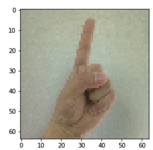
从上面可见测试的效果不是很好，之后优化下，使用dropout，感觉训练结果过拟合