Pytorch_Part1_简介&张量

VisualPytorch beta发布了！

功能概述：通过可视化拖拽网络层方式搭建模型，可选择不同数据集、损失函数、优化器生成可运行pytorch代码

扩展功能：1. 模型搭建支持模块的嵌套；2. 模型市场中能共享及克隆模型；3. 模型推理助你直观的感受神经网络在语义分割、目标探测上的威力；4.添加图像增强、快速入门、参数弹窗等辅助性功能

修复缺陷：1.大幅改进UI界面，提升用户体验；2.修改注销不跳转、图片丢失等已知缺陷；3.实现双服务器访问，缓解访问压力

访问地址：http://sunie.top:9000

发布声明详见：https://www.cnblogs.com/NAG2020/p/13030602.html

一、Pytorch简介与安装

1. 简介

PyTorch是在Torch基础上用python语言重新打造的一款深度学习框架.增长速度与TensorFlow一致.

2. 优点：

• 上手快：掌握Numpy和基本深度学习概念即可上手
• 代码简洁灵活：用nn.module封装使网络搭建更方便；基于动态图机制，更灵活
• Debug方便：调试PyTorch就像调试 Python 代码一样简单
• 文档规范：https: //pytorch.org/docs/ 可查各版本文档
• 资源多：arXiv中的新算法大多有PyTorch实现
• 开发者多：GitHub上贡献者(Contributors) 已超过1100+
• 背靠大树：FaceBook维护开发

3. 安装：

• anaconda(需添加中科大镜像)

• pycharm(将jetbrains-agent.jar 放 到安装目录\bin文件 夹，在 pycharm64.exe.vmoptions 中添加 命令 -javaagent:安装目录\jetbrains-agent.jar . 重启选择网页激活)

• pytorch(先安装cuda10.0及对应CuDNN版本，通过nvcc -V验证. 登陆https://download.pytorch.org/whl/torch_stable.html. 下载cu100/torch-1.2.0-cp37-cp37m-win_amd64.whl 及对应 torchvision 的whl文件，进入相应虚拟环境，先创建虚拟环境，再通过pip安装)。最后通过下面指令验证GPU版本Pytorch可以运行：

In [1]: import torch

In [2]: torch.cuda.current_device()
Out[2]: 0

In [3]: torch.cuda.device(0)
Out[3]: <torch.cuda.device at 0x7efce0b03be0>

In [4]: torch.cuda.device_count()
Out[4]: 1

In [5]: torch.cuda.get_device_name(0)
Out[5]: 'GeForce GTX 950M'

In [5]: torch.__version__
Out[5]: '1.2.0'

二、张量简介与创建

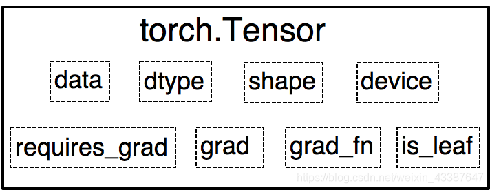
1. Tensor属性

0.4.0之前，Variable是torch.autograd中的数据类型，主要用于封装Tensor，进行自动求导，包含：

• data : 被包装的Tensor
• grad: data的梯度
• grad_fn : 创建Tensor的Function，是自动求导的关键
• requires_ grad : 指示是否需要梯度
• is_ leaf: 指示是否是叶子结点（张量）

之后的Tensor兼容了Variable的所有属性，并添加了下面三个：

• dtype : 张量的数据类型，如 torch .FloatTensor, torch.cuda.FloatTensor
• shape : 张量的形状，如( 64, 3, 224, 224 )
• device : 张量所在设备，GPU /CPU，是加速的关键

2. 创建

A. 直接

torch.tensor(data, dtype=None, device=None, requires_grad=False, pin_memory=False) # 是否锁页内存

torch.from_numpy(...) # 共享内存，参数同上

B. 依据数值

torch.zeros(*size, out=None, dtype=None, layout=torch.strided,device=None, requires_grad=False)
torch.zeros_like(input, dtype=None,layout=None,device=None, requires_grad=False)

torch.ones(...) # 参数同zeros
torch.ones_like(...) # 参数同zeros_like

# 以下函数参数从out起同zeros
torch.full(size, fill_value, ...)
torch.arange(start=0, end, step=1, ...) # step表步长

torch.linspace(start, end, steps=100, ...) # steps表长度 (steps-1)*step=end-start
torch.logspace(start, end, steps=100, base=10.0,...)
torch.eye(n, m=None,..)	# 二维，n行m列

C. 依据概率分布

torch.normal(mean, std, (size,) out=None) # mean, std 均为标量时size表示输出一维张量大小，否则没有size，输出的张量来自于不同分布

torch.randn(*size, out=None, dtype=None, layout=torch.strided,device=None, requires_grad=False) # 标准正太分布

torch.rand(...) # 均匀分布，参数同randn
torch.randint(low=0, high,...) # 均匀整数分布，参数从size同randn

torch.randperm(n,...) # 0到n-1随机排列，参数从out同randn
torch.bernoulli(input, *, generator=None, out=None) # 以input为概率，生成伯努力分布

三、张量操作与线性回归

1. 张量操作

A. 拼接与切分

torch.cat(tensors, dim=0, out=None)
torch.stack(tensors, dim=0, out=None) # 在新维度上拼接

torch.chunk(input, chunks, dim=0)
torch.split(tensor, split_size_or_sections, dim=0)

B. 张量索引

torch.index_select(input, dim, index, out=None)
torch.masked_select(input, mask, out=None) # mask为与input同形状的bool

C. 张量变换

torch.reshape(input, shape)
torch.transpose(input, dim0, dim1) # 交换的两维
torch.t(input)

torch.squeeze(input, dim=None, out=None) # 默认去除所有长度1的维，否则去除指定且长度为1的维
torch.usqueeze(input, dim, out=None)

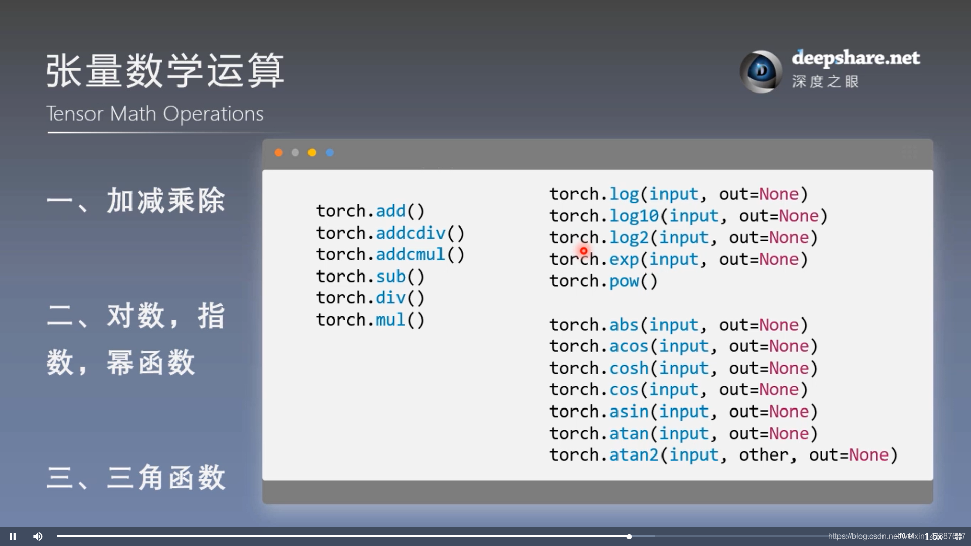
2. 数学运算

3. 线性回归

结果：

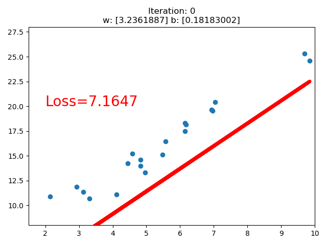
import torch
import matplotlib.pyplot as plt
torch.manual_seed(10)

lr = 0.05  # 学习率    20191015修改

# 创建训练数据
x = torch.rand(20, 1) * 10  # x data (tensor), shape=(20, 1)
y = 2*x + (5 + torch.randn(20, 1))  # y data (tensor), shape=(20, 1)

# 构建线性回归参数
w = torch.randn((1), requires_grad=True)
b = torch.zeros((1), requires_grad=True)

for iteration in range(1000):

    # 前向传播
    wx = torch.mul(w, x)
    y_pred = torch.add(wx, b)

    # 计算 MSE loss
    loss = (0.5 * (y - y_pred) ** 2).mean()

    # 反向传播
    loss.backward()

    # 更新参数
    b.data.sub_(lr * b.grad)
    w.data.sub_(lr * w.grad)

    # 清零张量的梯度   20191015增加
    w.grad.zero_()
    b.grad.zero_()

    # 绘图
    if iteration % 20 == 0:

        plt.scatter(x.data.numpy(), y.data.numpy())
        plt.plot(x.data.numpy(), y_pred.data.numpy(), 'r-', lw=5)
        plt.text(2, 20, 'Loss=%.4f' % loss.data.numpy(), fontdict={'size': 20, 'color':  'red'})
        plt.xlim(1.5, 10)
        plt.ylim(8, 28)
        plt.title("Iteration: {}\nw: {} b: {}".format(iteration, w.data.numpy(), b.data.numpy()))
        plt.pause(0.5)

        if loss.data.numpy() < 1:
            break

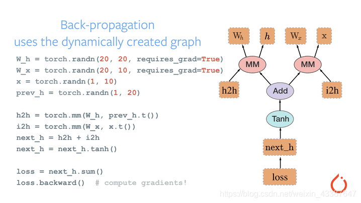
四、计算图与动态图机制

1. 计算图

计算图是用来描述运算的有向无环图，有两个主要元素：结点（Node，表示数据，如向量，矩阵，张量） 和边（Edge，表示运算，如加减乘除卷积等）结

用计算图表示：y = (x+ w) * (w+1) 如下

a = x + w
b = w + 1
y = a * b

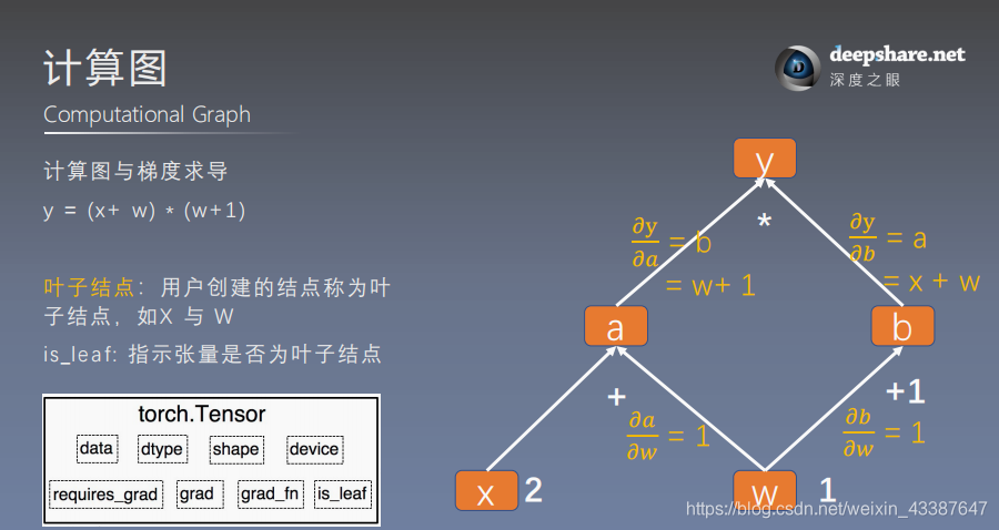
可以根据计算图构建相应的张量并计算梯度：

• 叶子张量：由用户创建的张量，保存梯度，没有梯度函数
• 非叶子张量：通过计算得到，反向传播会释放梯度。除非在反向传播之前a.retain_grd()

例如x=2 w=1 时，通过计算图得：

\(dw = \frac{\partial y}{\partial w} = \frac{\partial y}{\partial a} \frac{\partial a}{\partial w} + \frac{\partial y}{\partial b} \frac{\partial b}{\partial w} = b *1+a*1=w+1+x+w=5\)

w = torch.tensor([1.], requires_grad=True)
x = torch.tensor([2.], requires_grad=True)

a = torch.add(w, x)     # retain_grad()
b = torch.add(w, 1)
y = torch.mul(a, b)

y.backward()	# 张量内部方法，调用了torch.autograd.backward()
print(w.grad)

tensor([5.])

# 查看叶子结点
print("is_leaf:\n", w.is_leaf, x.is_leaf, a.is_leaf, b.is_leaf, y.is_leaf)

# 查看梯度
print("gradient:\n", w.grad, x.grad, a.grad, b.grad, y.grad)

# 查看 grad_fn
print("grad_fn:\n", w.grad_fn, x.grad_fn, a.grad_fn, b.grad_fn, y.grad_fn)

is_leaf:

True True False False False

gradient:

tensor([5.]) tensor([2.]) None None None

grad_fn:

None None <AddBackward0 object at 0x000001F6AABCB0F0> <AddBackward0 object at 0x000001F6C1A52048> <MulBackward0 object at 0x000001F6AACD7D68>

2. 动态图——运算与搭建同时

动态图vs静态图——自由行（灵活易调）vs跟团游

五、autograd与逻辑回归

1. autograd自动求取梯度

torch.autograd.backward(tensors,grad_tensors=None,retain_graph=None,create_graph=False)	

torch.autograd.grad(outputs,inputs,grad_outputs=None,retain_graph=None,create_graph=False) # 求指定inputs的梯度

Parameter:

• retain_graph 保存计算图，可多次

  w = torch.tensor([1.], requires_grad=True)
  x = torch.tensor([2.], requires_grad=True)
  
  a = torch.add(w, x)
  b = torch.add(w, 1)
  y = torch.mul(a, b)
  
  y.backward(retain_graph=True)
  # print(w.grad)
  y.backward()
  

• grad_tensors 表示多梯度权重

  y0 = torch.mul(a, b)    # y0 = (x+w) * (w+1)
  y1 = torch.add(a, b)    # y1 = (x+w) + (w+1)    dy1/dw = 2
  
  loss = torch.cat([y0, y1], dim=0)       # [y0, y1]
  
  loss.backward(gradient=torch.tensor([1., 2.]))    
  
  print(w.grad) # 1*5+2*2=9
  

• create_graph 输出为张量的元组，代表一种求导运算：

  x = torch.tensor([3.], requires_grad=True)
  y = torch.pow(x, 2)     # y = x**2
  
  grad_1 = torch.autograd.grad(y, x, create_graph=True)   # grad_1 = dy/dx = 2x = 2 * 3 = 6
  print(grad_1)
  
  grad_2 = torch.autograd.grad(grad_1[0], x)              # grad_2 = d(dy/dx)/dx = d(2x)/dx = 2
  print(grad_2)
  

  (tensor([6.], grad_fn=),)
  
  (tensor([2.]),)

Note:

• 梯度不自动清零

  w = torch.tensor([1.], requires_grad=True)
  x = torch.tensor([2.], requires_grad=True)
  
  for i in range(4):
      a = torch.add(w, x)
      b = torch.add(w, 1)
      y = torch.mul(a, b)
  
      y.backward()
      print(w.grad)
  

  如果没有 w.grad.zero_() ，梯度将会累积

• 依赖于叶子结点的结点，requires_grad默认为True

  print(a.requires_grad, b.requires_grad, y.requires_grad)
  

  True True True

• 叶子结点不可执行in-place

  a = torch.ones((1, ))
  a = a + torch.ones((1, ))	# a存储位置改变，为inplace操作
  a += torch.ones((1, ))
  

  w = torch.tensor([1.], requires_grad=True)
  x = torch.tensor([2.], requires_grad=True)
  
  a = torch.add(w, x)
  b = torch.add(w, 1)
  y = torch.mul(a, b)
  
  w.add_(1)
  
  y.backward()
  

  RuntimeError: a leaf Variable that requires grad has been used in an in-place operation.

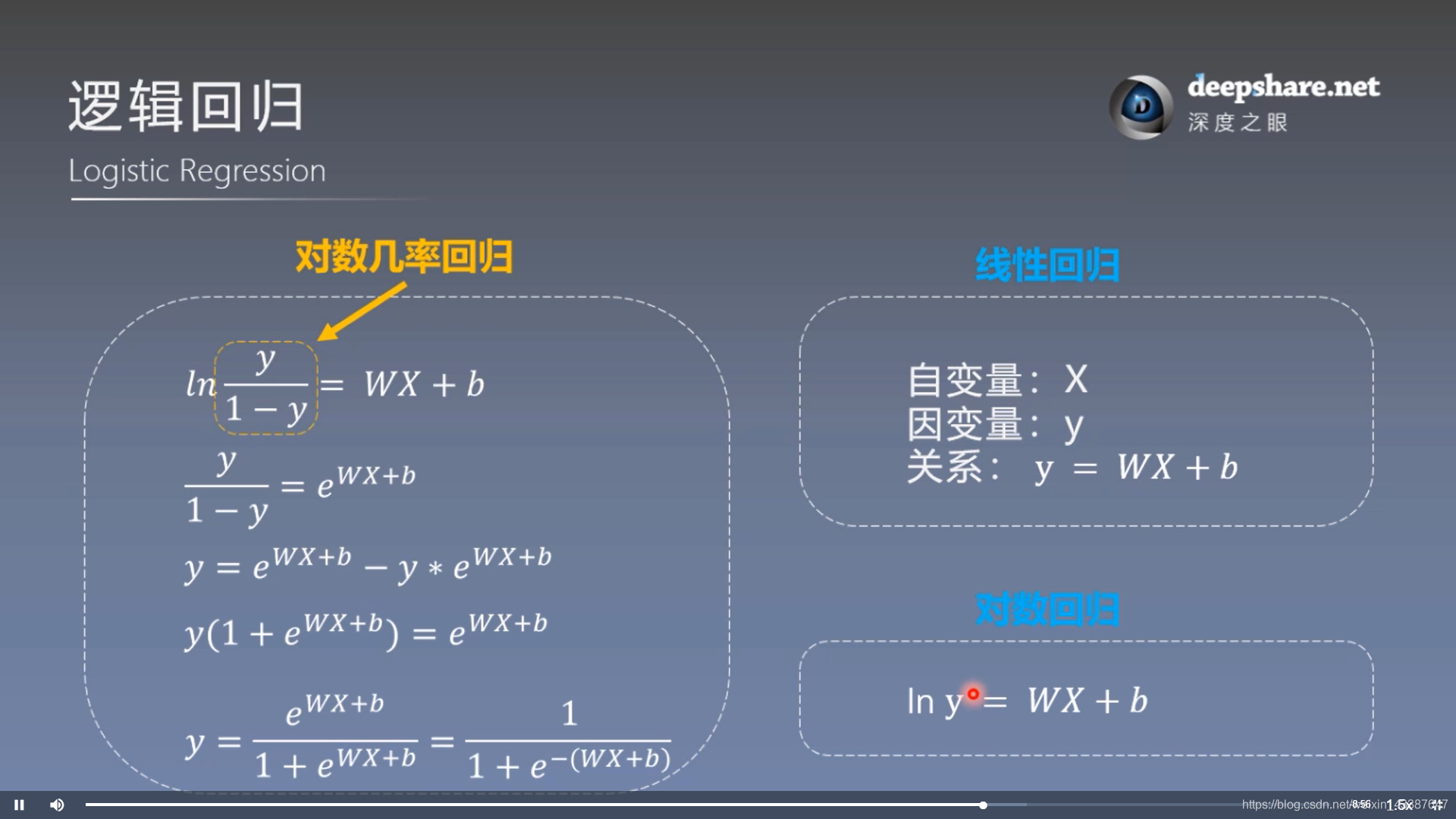
2. 逻辑回归 = 对数几率回归

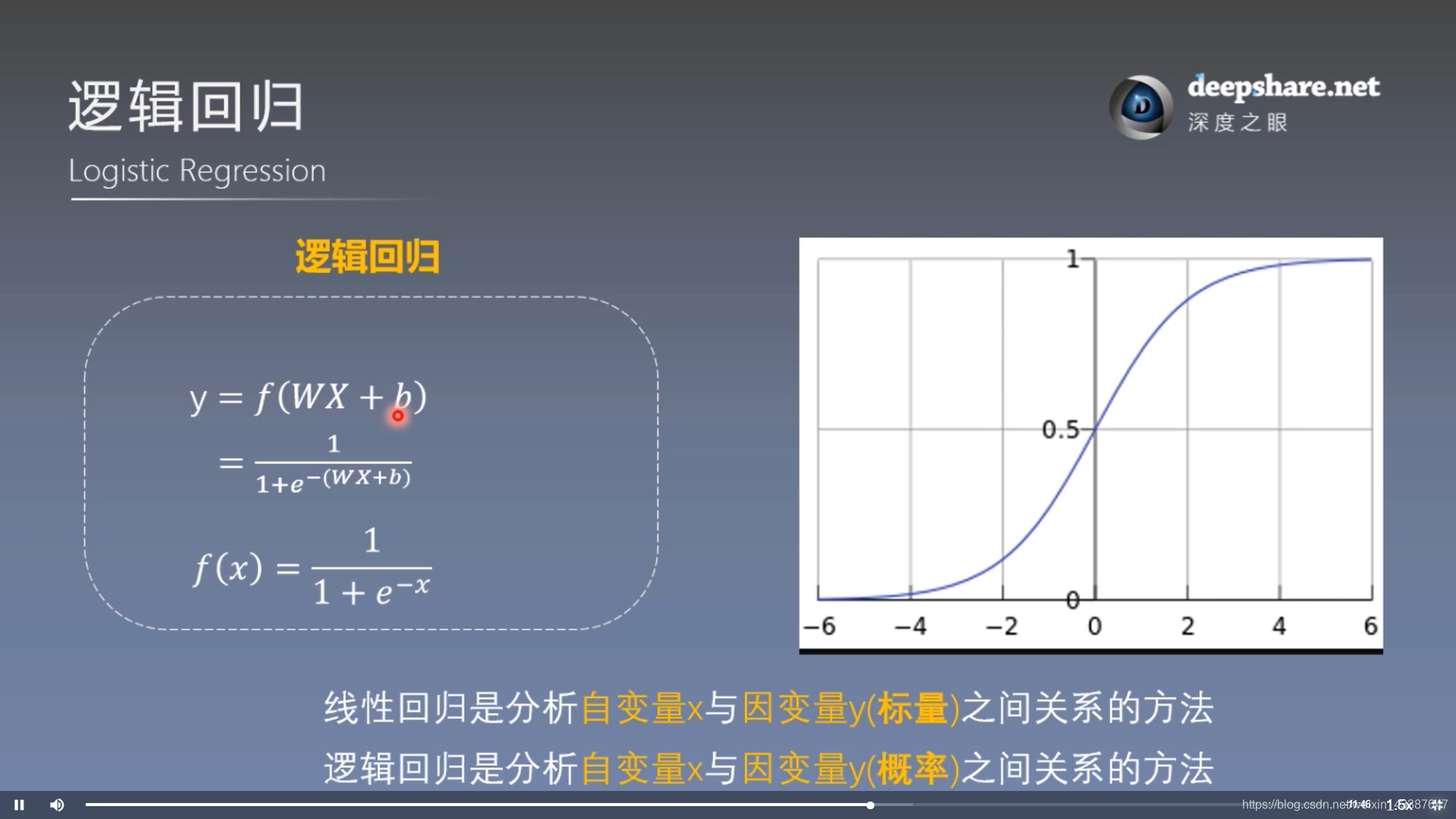
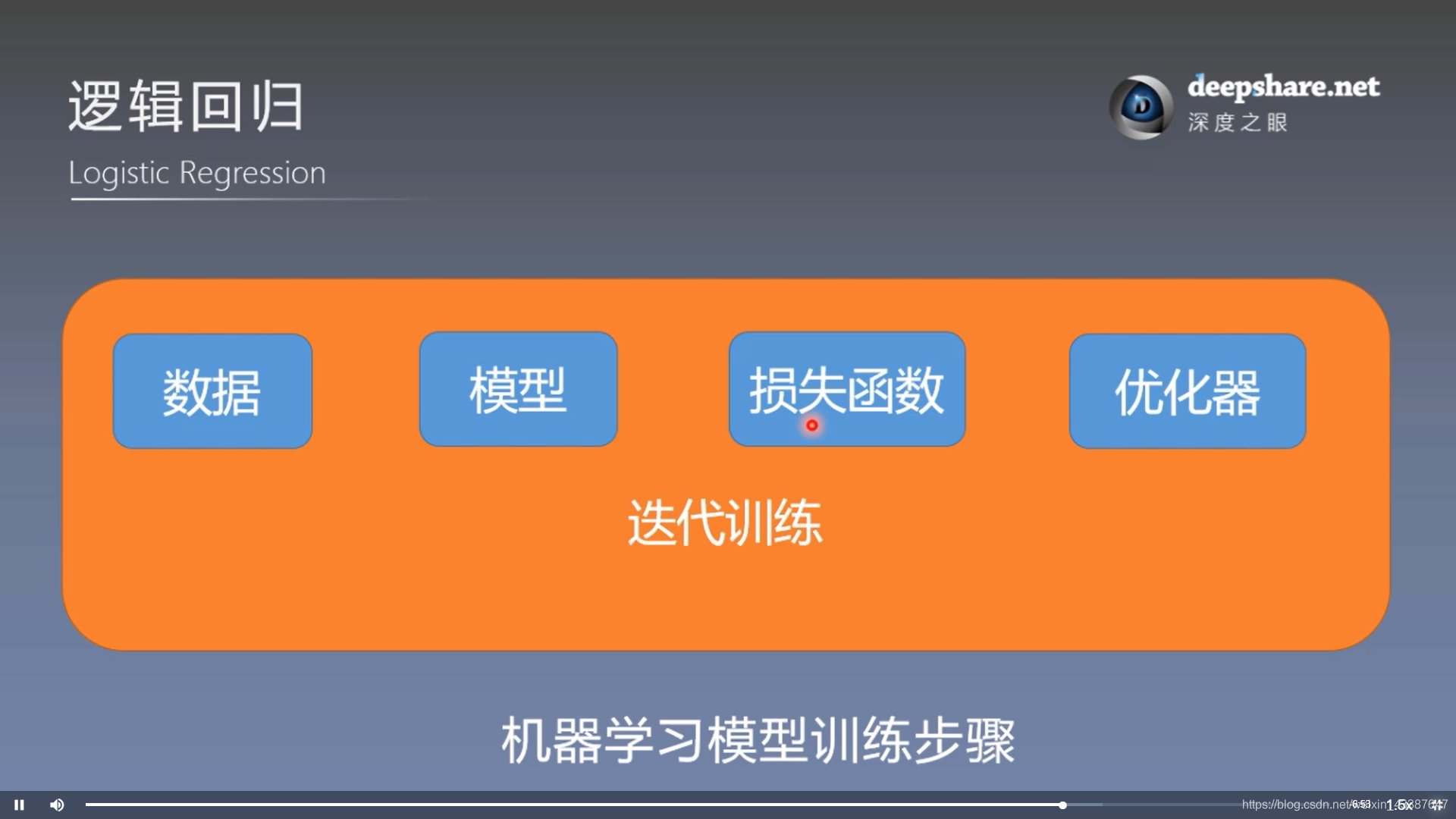
模型训练步骤：

结果：

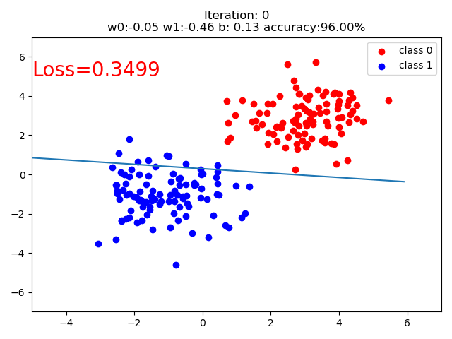
代码：

import torch
import torch.nn as nn
import matplotlib.pyplot as plt
import numpy as np
torch.manual_seed(10)

# ============================ step 1/5 生成数据 ============================
sample_nums = 100
mean_value = 1.7
bias = 1
n_data = torch.ones(sample_nums, 2)
x0 = torch.normal(mean_value * n_data, 1) + bias      # 类别0 数据 shape=(100, 2)
y0 = torch.zeros(sample_nums)                         # 类别0 标签 shape=(100, 1)
x1 = torch.normal(-mean_value * n_data, 1) + bias     # 类别1 数据 shape=(100, 2)
y1 = torch.ones(sample_nums)                          # 类别1 标签 shape=(100, 1)
train_x = torch.cat((x0, x1), 0)
train_y = torch.cat((y0, y1), 0)

# ============================ step 2/5 选择模型 ============================
class LR(nn.Module):
    def __init__(self):
        super(LR, self).__init__()
        self.features = nn.Linear(2, 1)
        self.sigmoid = nn.Sigmoid()

    def forward(self, x):
        x = self.features(x)
        x = self.sigmoid(x)
        return x

lr_net = LR()   # 实例化逻辑回归模型

# ============================ step 3/5 选择损失函数 ============================
loss_fn = nn.BCELoss()

# ============================ step 4/5 选择优化器   ============================
lr = 0.01  # 学习率
optimizer = torch.optim.SGD(lr_net.parameters(), lr=lr, momentum=0.9)

# ============================ step 5/5 模型训练 ============================
for iteration in range(1000):

    # 前向传播
    y_pred = lr_net(train_x)

    # 计算 loss
    loss = loss_fn(y_pred.squeeze(), train_y)

    # 反向传播
    loss.backward()

    # 更新参数
    optimizer.step()

    # 清空梯度
    optimizer.zero_grad()

    # 绘图
    if iteration % 20 == 0:

        mask = y_pred.ge(0.5).float().squeeze()  # 以0.5为阈值进行分类
        correct = (mask == train_y).sum()  # 计算正确预测的样本个数
        acc = correct.item() / train_y.size(0)  # 计算分类准确率

        plt.scatter(x0.data.numpy()[:, 0], x0.data.numpy()[:, 1], c='r', label='class 0')
        plt.scatter(x1.data.numpy()[:, 0], x1.data.numpy()[:, 1], c='b', label='class 1')

        w0, w1 = lr_net.features.weight[0]
        w0, w1 = float(w0.item()), float(w1.item())
        plot_b = float(lr_net.features.bias[0].item())
        plot_x = np.arange(-6, 6, 0.1)
        plot_y = (-w0 * plot_x - plot_b) / w1

        plt.xlim(-5, 7)
        plt.ylim(-7, 7)
        plt.plot(plot_x, plot_y)

        plt.text(-5, 5, 'Loss=%.4f' % loss.data.numpy(), fontdict={'size': 20, 'color': 'red'})
        plt.title("Iteration: {}\nw0:{:.2f} w1:{:.2f} b: {:.2f} accuracy:{:.2%}".format(iteration, w0, w1, plot_b, acc))
        plt.legend()

        plt.show()
        plt.pause(0.5)

        if acc > 0.99:
            break