论文解读二代GCN《Convolutional Neural Networks on Graphs with Fast Localized Spectral Filtering》

Paper Information

Title：Convolutional Neural Networks on Graphs with Fast Localized Spectral Filtering
Authors：Michaël DefferrardXavier BressonPierre Vandergheynst
Paper：Download 
Source：NeurIPS 2016

---

Abstract

　　基于   spectral graph theory  ，为设计 localized convolutional filters on graphs  提供了必要的数学背景和有效的数值方案。

　　Our method's advantages：

• • The proposed technique offers  linear computational complexity.
  • Constant learning complexity.

---

Review

　　At the begining ,we just do a review about the first generation GCN.

　　　　$x_{k+1, j}=h\left(V \sum \limits _{i=1}^{f_{k-1}} F_{k, i, j} V^{T} x_{k, i}\right) \quad\left(j=1 \ldots f_{k}\right)$

　　其中，$F(k,i,j)$ 是图卷积神经网络在第  $k$  层的 filter ，可学习，具有任意性。由图卷积公式可以看出，卷积核不具备局部性，并且依赖于图的 Laplacian 的谱分解。

---

1 Introduction

　　CNN的优势：

• • Offer an efficient architecture to extract highly meaningful statistical patterns in large-scale and high-dimensional datasets.
  • Can learn  local stationary structures.
  • Can  compose the local stationary structures to form multi-scale hierarchical patterns in many domain.

　　What CNN do?

• • CNNs extract the local stationarity property of the input data or signals by revealing local features that are shared across the data domain.
  • Similar features are identifified with localized convolutional fifilters or kernels,which are learned from the data.

　　Why CNN can recognize identical features independently of their spatial locations?

• • Due to  Convolutional filters are shift  or translation-invariant filters.

　　Then,explain the common of  non-Euclidean data ,such as social networks, gene data on biological regulatory networks, log data on telecommunication networks, or text documents on word embeddings

　　Why CNN can't apply in graph directly?

• • The convolution and pooling operators are only defined for regular grids.
  • Major bottleneck : how to  define a localized graph filters which are efficient to evaluate and learn.

　　Main contributions as the following:

• • Spectral formulation. If you have the ability ,you can read this paper at first.——《 The Emerging Field of Signal Processing on Graphs: Extending High-Dimensional Data Analysis to Networks and other Irregular Domains》
  • Strictly localized fifilters. 本文提出的  spectral filters 在以中心节点的为半径的最短路径内是严格局部化的。
  • Low computational complexity.  本文提出的卷积核的复杂度是和卷积核的尺寸以及边的数量成线性关系的，另外由于大多数图稀疏的，我们可以估计地认为  $|\varepsilon| \ll n^{2} $  并且  $|\varepsilon|=k n$ ，也就是每个节点只和  $k$  个近邻有边，这样复杂度就和节点数量成线性关系。另外本方法避免了使用 Fourier basis，因此不再需要进行昂贵的  EVD (特征值分解) 以及存储  Fourier basis（使用一个大小的矩阵）。除了数据，本方法只需要存储  Laplacian matrix 这个包含  $|\mathcal{E}|$  non-zero values  的  sparse 矩阵。
  • Efficient pooling. 将顶点重新排列为一个二叉树结构。
  • Experimental results. 通过实验证明了方法的有效性，并与其他方法进行了对比。

---

2 Proposed Technique

　　 Generalizing CNNs to graphs requires three fundamental steps:

1. 1. the design of localized convolutional filters on graphs（局部卷积核设置）;
   2. a graph coarsening procedure that groups together similar vertices （图的粗化）;
   3. a graph pooling operation that trades spatial resolution for higher filter resolution（图的池化）.

2.1 Learning Fast Localized Spectral Filters

　　Two strategies to define convolutional filters:

• • from a spatial approach.
  • from a spectral approach.

　　Why not choose spatial approach?

• • Although graph convolution in the spatial domain is conceivable, it faces the challenge of matching local neighborhoods .
  • No unique mathematical definition of translation on graphs from a spatial perspective.

　　Spectral filter's challenge：

• • 频域卷积核需要借助  convolutions with a Kronecker delta implemented ；
  • 由于要与  Graph Fourier basis 相乘，会产生  $O\left(n^{2}\right)$  的复杂度，转换成本高。

2.1.1 Graph Fourier Transform

　　$ x: \mathcal{V}  \rightarrow \mathbb{R}$ defined on the nodes of the graph may be regarded as a vector  $x \in \mathbb{R}^{n}$  where  $x_{i}$  is the value of  $x$  at the  $i^{t h}$  node.

　　graph Laplacian ：$L=U \Lambda U^{T} $　($L=D-W \in \mathbb{R}^{n \times n}$ or $L=I_{n}-D^{-1 / 2} W D^{-1 / 2}$)

　　where

• • $L$  is a real symmetric positive semidefinite matrix.
  • Fourier basis  $U=\left[u_{0}, \ldots, u_{n-1}\right] \in \mathbb{R}^{n \times n}$.
  • orthonormal eigenvectors  $\left\{u_{l}\right\}_{l=0}^{n-1} \in \mathbb{R}^{n}$ and nonnegative eigenvalues  $\left\{\lambda_{l}\right\}_{l=0}^{n-1}$ .
  • $\Lambda=\operatorname{diag}\left(\left[\lambda_{0}, \ldots, \lambda_{n-1}\right]\right) \in \mathbb{R}^{n \times n}$ .

　　A signal  $x \in \mathbb{R}^{n}$  is then defined as  $\hat{x}=U^{T} x \in \mathbb{R}^{n}$ , and its inverse as  $x=U \hat{x}$ .

2.1.2 Spectral filtering of graph signals

　　由于很难在 vertex domain （理解为空域）  定义一个  translation operator，所以考虑在  graph 上借由  Fourier domain  （理解为频域）去定义一个   convolution operator  。这里将两个图信号的卷积操作记作：

　　　　$x *_{G} y=U\left(\left(U^{T} x\right) \odot\left(U^{T} y\right)\right)$

　　将图信号  $x$  的经过  $g_{\theta}$  卷积，写成：

　　　　$y=g_{\theta}(L) x=g_{\theta}\left(U \Lambda U^{T}\right) x=U g_{\theta}(\Lambda) U^{T} x$

　　其中

　　　　$g_{\theta}(\Lambda)=\operatorname{diag}(\theta)$ 

　　是特征值的对角矩阵。一个非参数化（non-parametric）的卷积核，也就是说它的参数全部都是自由参数。

　　这里  $\theta \in \mathbb{R}^{n}$  ，是一个傅里叶系数向量，其实可以理解为卷积核与相乘后的结果，这个结果的每一维相当于这一维对应的特征向量的系数。

其他解释：

　　图上的傅里叶变换与逆变换为：

　　　　$\begin{array}{l}\hat{f}=U^{T} f \\f=U \hat{f}\end{array}$

　　根据傅里叶变换与卷积的关系，为了导出图卷积公式，我们先计算图与卷积核的傅里叶变换，再将其相乘，最后求其逆变换：

　　　　$f * g=\mathscr{F}^{-1}(\mathscr{F}(f) \mathscr{F}(g))$

　　带入可得：

　　　　$f * g=U\left(\left(U^{T} f\right) \odot\left(U^{T} g\right)\right)$

　　这里对于卷积核的傅里叶变换我们可以写为：

　　　　$U^{T} g=\left(\hat{g}\left(\lambda_{1}\right), \hat{g}\left(\lambda_{2}\right), \ldots, \hat{g}\left(\lambda_{n}\right)\right)^{T}$

　　故可将哈达马积去掉，写成：

　　　　$f * g=U \operatorname{diag}\left(\hat{g}\left(\lambda_{1}\right), \hat{g}\left(\lambda_{2}\right), \ldots, \hat{g}\left(\lambda_{n}\right)\right) U^{T} f$

2.1.3  Polynomial parametrization for localized filters.

　　前述非参数化的卷积核有两个局限性：

1. 1. 这样的卷积核在空间上不是局部化的；
   2. 学习复杂度是  $O(n)$。

　　这些问题可以通过使用多项式滤波器来解决

　　　　$g_{\theta}(\Lambda)=\sum \limits _{k=0}^{K-1} \theta_{k} \Lambda^{k}$

　　其中 $\theta \in \mathbb{R}^{K} $ ，是多项式的系数向量，是要学习的参数。此时，图信号被  $g_{\theta}$  所卷积后得到的结果为:

　　　　$\begin{array}{l}y&=U\left(\sum \limits _{k=0}^{K-1} \theta_{k} \Lambda^{k}\right) U^{T} x \\&=\left(\sum \limits_{k=0}^{K-1} \theta_{k} U \Lambda^{k} U^{T}\right) x \\&=\sum \limits_{k=0}^{K-1} \theta_{k} L^{k} x\end{array}$

　　经证明，当  $d_{G}(i, j)>K$  时有  $\left(L^{K}\right)_{i, j}=0$， 其中  $ d_{G}$  代表最短路径距离。此时就说这样的卷积核是严格 K-localized 的。另外，学习参数复杂度为  $O(K)$  ，与 CNN相同。

　　此种卷积核有以下特点:

1. 1. 卷积核只有  $K$  个参数，一般  $K \ll n$   ，参数复杂度大大降低；
   2. 不需要进行拉普拉斯矩阵的特征分解，直接使用拉普拉斯矩阵进行变换，然而由于要计算  $K$   次，计算复杂度还是   $O\left(n^{3}\right)$ ;
   3. 卷积核具有很好的空间局部性（就是卷积核的感受野），也就是说每次卷积会将中心顶点  K-hop neighbor  上的  feature  进行加权求和，权系数就是   $\theta_{k} $。

2.1.4 Recursive formulation for fast filtering.

　　非参数化的卷积核的复杂度较高，并且上述多项式卷积核的计算复杂度仍然是比较高的。

　　本小节介绍的卷积核应用切比雪夫多项式，能够实现由于使用非参数化的卷积核复杂度较高，且多项式卷积核的计算复杂度依然差不多。思路是将  $g_{\theta}(L)$  参数化为一个可由递归计算的多项式函数，这样的多项式可以采用切比雪夫多项式，如下：

　　　　$\begin{array}{l}T_{0}(x)=1 \\T_{1}(x)=x \\T_{k}(x)=2 x T_{k-1}(x)-T_{k-2}(x)\end{array}$

　　参考：《 切比雪夫多项式》

　　利用切比雪夫多项式，卷积核设计为：

　　　　$g_{\theta}(\Lambda)=\sum \limits _{k=0}^{K-1} \theta_{k} T_{k}(\widetilde{\Lambda})$

　　其中，  $\theta_{k}$  是切比雪夫系数向量，也就是需要学习的参数。$T_{k}(\widetilde{\Lambda}) \in \mathbb{R}^{n \times n}$  是阶的切比雪夫多项式，  $\widetilde{\Lambda}=2 \Lambda / \lambda_{\max }-I_{n}$  ，这样可以将特征值标准化到之间。

　　如此卷积操作就是下面这样的过程:

　　　　$y=g_{\theta}(L) x=\sum \limits _{k=0}^{K-1} \theta_{k} T_{k}(\widetilde{L}) x$

　　上式的推导过程很简单就不赘述了，这里的  $\widetilde{L} \in \mathbb{R}^{n \times n}$  也就是标准化以后的，即  $\widetilde{L}=2 L / \lambda_{\max }-I_{n} $ 。
　　将  $\bar{x}_{k}$  记作  $\bar{x}_{k}=T_{k}(\widetilde{L}) x \in \mathbb{R}^{k}$  ，同样地也可以利用递归关系去计算  $\bar{x}_{k}=2 \widetilde{L} \bar{x}_{k-1}-\bar{x}_{k-2} $  ，此时  $\bar{x}_{0}=x, \bar{x}_{1}=\widetilde{L} x $ ，此时卷积的过程又可以表示为:

　　　　$y=g_{\theta}(L) x=\left[\bar{x}_{0}, \cdots, \bar{x}_{K-1}\right] \theta$

　　这样设计的卷积过程的复杂度为  $O(K|\varepsilon|) $ 。对比上一小节的多项式卷积核，这里利用切比雪夫多项 式设计的卷积核不再需要计算，而只是利用仅包含加减操作的递归关系来计算  $T_{k}(\widetilde{L})$  ，这样大大减少了计算的复杂度。

2.1.5  Learning filters

　　在一个卷积层中，一个样本的第个  $j^{\text {th }}$   feature map 的输出为：

　　　　$y_{s, j}=\sum \limits _{i=1}^{F_{i n}} g_{\theta_{i, j}}(L) x_{s, i} \in \mathbb{R}^{n}$

　　 $x_{s, i}$  是输入的feature map，总计有  $F_{\text {in }} \times F_{\text {out }}$  个向量  $\theta_{i, j} $ ，这些是需要学习的参数向量。 另外在训练时需要计算两个梯度：

　　　　$\begin{array}{l}\frac{\partial E}{\partial \theta_{i, j}}=\sum \limits _{s=1}^{S}\left[\bar{x}_{s, i, 0}, \cdots, \bar{x}_{s, i, K-1}\right]^{T} \frac{\partial E}{\partial y_{s, j}} \\\frac{\partial E}{\partial x_{s, i}}=\sum \limits_{j=1}^{F_{\text {out }}} g_{\theta_{i, j}}(L) \frac{\partial E}{\partial y_{s, j}}\end{array}$

　　是损失函数，由于采用多项式卷积核，不同阶直接是累加关系，因此无论是计算对还是的梯度，都只需要先计算对的梯度，再利用累加关系很方便地就能得到最终结果，因此应用反向传播算法学习参数是可行的，在并行运算时也是高效的。还有一点就是   $ \left[\bar{x}_{s, i, 0}, \cdots, \bar{x}_{s, i, K-1}\right] $  只需要计算一次。

2.2 Graph Coarsening

　　池化操作需要将相似的节点聚类到一起，对于多层网络来说做到这一点相当于对需要保持局部几何 结构的图进行多尺度聚类（multi-scale clustering）。图的聚类方法存在多种，比如常见的谱聚类 方法（参考链接：谱聚类|机器学习推导系列 (二十) )。在本文的方法中没有采用谱聚类这种方 法，而是选择了一种近似能够将图的规模除以2的聚类方法，这样的方法可以精确控制粗化和池化的 size。本文采用的图粗化方法为Graclus多尺度聚类算法。

　　Graclus方法采用一种贪婪的方法来计算给定图的连续的粗化的版本，并且能够最小化多种谱聚类 的目标，在这里选择的目标为normalized cut。具体的方法是在每层进行粗化时，选择一个末标记 的节点，然后选择一个能够最小化   $W_{i j}\left(1 / d_{i}+1 / d_{j}\right)$  的末标记的邻居节点，然后将这两个节点标记，这两个匹配的节点在池化时被合并，合并节点的信号是这两个节点的信号加和。上述匹配的过程一直进行下去知道所有节点被遍历。这种方法是非常快速的，并且能够将图的规模近似除以2， 之所以近似是因为可能有一些末匹配的节点（文中称为singleton节点）。

2.3 Fast Pooling of Graph Signals

　　池化操作被执行多次，所以必须是高效的。输入的图和粗化图的节点的排列方法是无意义的，因此，一个直接的池化操作的方法是需要一张表来保存匹配的节点，然而这种方法是内存低效的，并且缓慢，也不能并行处理。本文采用的方法可以使得池化操作像1D池化那样高效。

　　本文采用的方法分两个步骤：
　　①创建一个平衡二叉树；
　　②重排列所有节点。

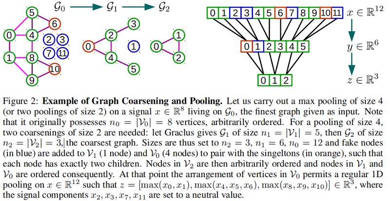
　　在进行图的粗化以后，粗化图的每个节点要么有两个子节点（被匹配到的节点），要么只有一个节点（singleton节点）。从最粗到最细的图，将会添加fake节点（不与图连接在一起）到每一层来与singleton节点进行匹配。这样的结构是一个平衡二叉树，主要包含3种节点：
　　①regular节点（或者singleton节点），拥有两个regular子节点（如下图 level 1节点0）；
　　②regular节点（或者singleton节点），拥有一个regular节点和一个singleton节点作为子节点的节点（如下图 level 2节点0）；
　　③fake节点，总是拥有两个fake子节点（如下图 level 1节点1）。

　　fake节点的值初始化通常选择一个中性的值，比如当使用max pooling和ReLU激活函数时初始化为0。这些fake节点不与图的节点连接，因此卷积操作不会影响到它们。虽然这些节点会增加数据的维度，这样会增加计算的花费，但是在实践中证明Graclus方法所剩下的singleton节点是比较少的。在最粗化的图中任意排列节点，然后传播回最细的图中，这是由于粗化图中第的节点的子节点是上一层图中的  $2k$  和   $2k+1$   节点，这样就可以在最细的图中有一个规范的排列顺序，这里规范是指相邻节点在较粗的层次上分层合并。这种  pooling  方法类似  1D pooling。这种规范的排列能够让  pooling  操作非常的高效且可以并行化，并且内存访问是  local 的。下图是这种方法的一个例子：

　　　　

---

3 Numerical Experiments

　　这里简单列几个实验结果，具体实验设置可以自行参考原论文。

　　1、MNIST数据集上对比经典CNN

　　　　

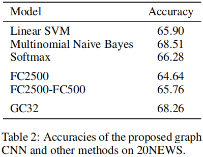
　　2、20NEWs数据集上多种架构效果

　　　　

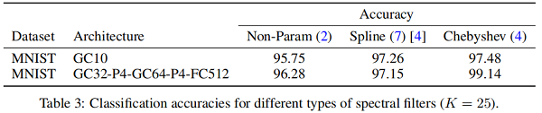
　　3、MNIST数据集上多种卷积核的对比

　　下图中Non-Param和Spline代表第一代GCN论文中提出的两种卷积核，Chebyshev代表本文提出的卷积核：

　　　　

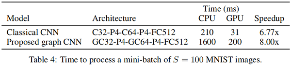
　　4、GPU加速效果对比

　　下图表明本文提出的GCN结构在使用GPU加速时比经典CNN能获得更多的加速倍数，说明该架构的并行化处理能力是比较可观的：