[机器学习&数据挖掘]机器学习实战决策树plotTree函数完全解析

在看机器学习实战时候，到第三章的对决策树画图的时候，有一段递归函数怎么都看不懂，因为以后想选这个方向为自己的职业导向，抱着精看的态度，对这本树进行地毯式扫描，所以就没跳过，一直卡了一天多，才差不多搞懂，才对那个函数中的plotTree.xOff的取值，以及计算cntrPt的方法搞懂，相信也有人和我一样，希望能够相互交流。

先把代码贴在这里：

import matplotlib.pyplot as plt

#这里是对绘制是图形属性的一些定义，可以不用管，主要是后面的算法
decisionNode = dict(boxstyle="sawtooth", fc="0.8")
leafNode = dict(boxstyle="round4", fc="0.8")
arrow_args = dict(arrowstyle="<-")

#这是递归计算树的叶子节点个数，比较简单
def getNumLeafs(myTree):
    numLeafs = 0
    firstStr = myTree.keys()[0]
    secondDict = myTree[firstStr]
    for key in secondDict.keys():
        if type(secondDict[key]).__name__=='dict':#test to see if the nodes are dictonaires, if not they are leaf nodes
            numLeafs += getNumLeafs(secondDict[key])
        else:   numLeafs +=1
    return numLeafs
#这是递归计算树的深度，比较简单
def getTreeDepth(myTree):
    maxDepth = 0
    firstStr = myTree.keys()[0]
    secondDict = myTree[firstStr]
    for key in secondDict.keys():
        if type(secondDict[key]).__name__=='dict':#test to see if the nodes are dictonaires, if not they are leaf nodes
            thisDepth = 1 + getTreeDepth(secondDict[key])
        else:   thisDepth = 1
        if thisDepth > maxDepth: maxDepth = thisDepth
    return maxDepth
#这个是用来一注释形式绘制节点和箭头线，可以不用管
def plotNode(nodeTxt, centerPt, parentPt, nodeType):
    createPlot.ax1.annotate(nodeTxt, xy=parentPt,  xycoords='axes fraction',
             xytext=centerPt, textcoords='axes fraction',
             va="center", ha="center", bbox=nodeType, arrowprops=arrow_args )
#这个是用来绘制线上的标注，简单
def plotMidText(cntrPt, parentPt, txtString):
    xMid = (parentPt[0]-cntrPt[0])/2.0 + cntrPt[0]
    yMid = (parentPt[1]-cntrPt[1])/2.0 + cntrPt[1]
    createPlot.ax1.text(xMid, yMid, txtString, va="center", ha="center", rotation=30)
#重点，递归，决定整个树图的绘制，难（自己认为）
def plotTree(myTree, parentPt, nodeTxt):#if the first key tells you what feat was split on
    numLeafs = getNumLeafs(myTree)  #this determines the x width of this tree
    depth = getTreeDepth(myTree)
    firstStr = myTree.keys()[0]     #the text label for this node should be this
    cntrPt = (plotTree.xOff + (1.0 + float(numLeafs))/2.0/plotTree.totalW, plotTree.yOff)

    plotMidText(cntrPt, parentPt, nodeTxt)
    plotNode(firstStr, cntrPt, parentPt, decisionNode)
    secondDict = myTree[firstStr]
    plotTree.yOff = plotTree.yOff - 1.0/plotTree.totalD
    for key in secondDict.keys():
        if type(secondDict[key]).__name__=='dict':#test to see if the nodes are dictonaires, if not they are leaf nodes
            plotTree(secondDict[key],cntrPt,str(key))        #recursion
        else:   #it's a leaf node print the leaf node
            plotTree.xOff = plotTree.xOff + 1.0/plotTree.totalW
            plotNode(secondDict[key], (plotTree.xOff, plotTree.yOff), cntrPt, leafNode)
            plotMidText((plotTree.xOff, plotTree.yOff), cntrPt, str(key))
    plotTree.yOff = plotTree.yOff + 1.0/plotTree.totalD
#if you do get a dictonary you know it's a tree, and the first element will be another dict

#这个是真正的绘制，上边是逻辑的绘制
def createPlot(inTree):
    fig = plt.figure(1, facecolor='white')
    fig.clf()
    axprops = dict(xticks=[], yticks=[])
    createPlot.ax1 = plt.subplot(111, frameon=False)    #no ticks
    plotTree.totalW = float(getNumLeafs(inTree))
    plotTree.totalD = float(getTreeDepth(inTree))
    plotTree.xOff = -0.5/plotTree.totalW; plotTree.yOff = 1.0;
    plotTree(inTree, (0.5,1.0), '')
    plt.show()

#这个是用来创建数据集即决策树
def retrieveTree(i):
    listOfTrees =[{'no surfacing': {0:{'flippers': {0: 'no', 1: 'yes'}}, 1: {'flippers': {0: 'no', 1: 'yes'}}, 2:{'flippers': {0: 'no', 1: 'yes'}}}},
                  {'no surfacing': {0: 'no', 1: {'flippers': {0: {'head': {0: 'no', 1: 'yes'}}, 1: 'no'}}}}
                  ]
    return listOfTrees[i]

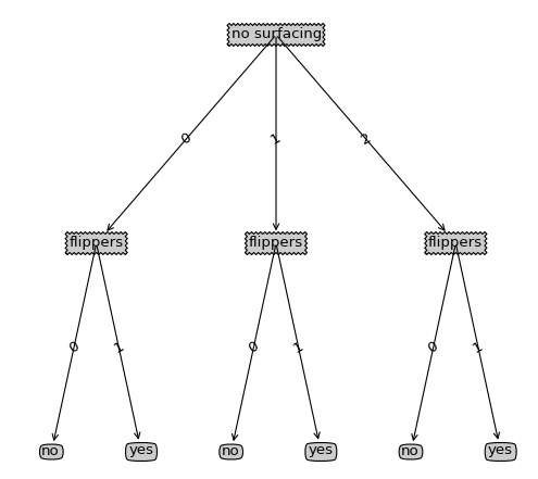
createPlot(retrieveTree(0))

绘制出来的图形如下：

先导：这里说一下为什么说一个递归树的绘制为什么会是很难懂，这里不就是利用递归函数来绘图么，就如递归计算树的深度、叶子节点一样，问题不是递归的思路，而是这本书中一些坐标的起始取值、以及在计算节点坐标所作的处理，而且在树中对这部分并没有取讲述，所以在看这段代码的时候可能大体思路明白但是具体的细节却知之甚少，所以本篇主要是对其中书中提及甚少的作详细的讲述，当然代码的整体思路也不会放过的

准备：这里说一下具体绘制的时候是利用自定义plotNode函数来绘制，这个函数一次绘制的是一个箭头和一个节点，如下图：

思路：这里绘图，作者选取了一个很聪明的方式，并不会因为树的节点的增减和深度的增减而导致绘制出来的图形出现问题，当然不能太密集。这里利用整棵树的叶子节点数作为份数将整个x轴的长度进行平均切分，利用树的深度作为份数将y轴长度作平均切分，并利用plotTree.xOff作为最近绘制的一个叶子节点的x坐标，当再一次绘制叶子节点坐标的时候才会plotTree.xOff才会发生改变;用plotTree.yOff作为当前绘制的深度，plotTree.yOff是在每递归一层就会减一份（上边所说的按份平均切分），其他时候是利用这两个坐标点去计算非叶子节点，这两个参数其实就可以确定一个点坐标，这个坐标确定的时候就是绘制节点的时候

整体算法的递归思路倒是很容易理解：

每一次都分三个步骤：

　　(1)绘制自身

　　(2)判断子节点非叶子节点，递归

　　(3)判断子节点为叶子节点，绘制

详细解析：

def plotTree(myTree, parentPt, nodeTxt):#if the first key tells you what feat was split on
    numLeafs = getNumLeafs(myTree)  #this determines the x width of this tree
    depth = getTreeDepth(myTree)
    firstStr = myTree.keys()[0]     #the text label for this node should be this
    cntrPt = (plotTree.xOff + (1.0 + float(numLeafs))/2.0/plotTree.totalW, plotTree.yOff)

    plotMidText(cntrPt, parentPt, nodeTxt)
    plotNode(firstStr, cntrPt, parentPt, decisionNode)
    secondDict = myTree[firstStr]
    plotTree.yOff = plotTree.yOff - 1.0/plotTree.totalD
    for key in secondDict.keys():
        if type(secondDict[key]).__name__=='dict':#test to see if the nodes are dictonaires, if not they are leaf nodes
            plotTree(secondDict[key],cntrPt,str(key))        #recursion
        else:   #it's a leaf node print the leaf node
            plotTree.xOff = plotTree.xOff + 1.0/plotTree.totalW
            plotNode(secondDict[key], (plotTree.xOff, plotTree.yOff), cntrPt, leafNode)
            plotMidText((plotTree.xOff, plotTree.yOff), cntrPt, str(key))
    plotTree.yOff = plotTree.yOff + 1.0/plotTree.totalD
#if you do get a dictonary you know it's a tree, and the first element will be another dict

def createPlot(inTree):
    fig = plt.figure(1, facecolor='white')
    fig.clf()
    axprops = dict(xticks=[], yticks=[])
    createPlot.ax1 = plt.subplot(111, frameon=False)    #no ticks
    plotTree.totalW = float(getNumLeafs(inTree))
    plotTree.totalD = float(getTreeDepth(inTree))
    plotTree.xOff = -0.5/plotTree.totalW; plotTree.yOff = 1.0;#totalW为整树的叶子节点树，totalD为深度
    plotTree(inTree, (0.5,1.0), '')
    plt.show()

上边代码中红色部分如此处理原理：

首先由于整个画布根据叶子节点数和深度进行平均切分，并且x轴的总长度为1,即如同下图：

1、其中方形为非叶子节点的位置，@是叶子节点的位置，因此每份即上图的一个表格的长度应该为1/plotTree.totalW,但是叶子节点的位置应该为@所在位置，则在开始的时候plotTree.xOff的赋值为-0.5/plotTree.totalW,即意为开始x位置为第一个表格左边的半个表格距离位置，这样作的好处为：在以后确定@位置时候可以直接加整数倍的1/plotTree.totalW,

2、对于plotTree函数中的红色部分即如下：

cntrPt = (plotTree.xOff + (1.0 + float(numLeafs))/2.0/plotTree.totalW, plotTree.yOff)

plotTree.xOff即为最近绘制的一个叶子节点的x坐标，在确定当前节点位置时每次只需确定当前节点有几个叶子节点，因此其叶子节点所占的总距离就确定了即为float(numLeafs)/plotTree.totalW*1(因为总长度为1)，因此当前节点的位置即为其所有叶子节点所占距离的中间即一半为float(numLeafs)/2.0/plotTree.totalW*1，但是由于开始plotTree.xOff赋值并非从0开始，而是左移了半个表格，因此还需加上半个表格距离即为1/2/plotTree.totalW*1,则加起来便为(1.0 + float(numLeafs))/2.0/plotTree.totalW*1，因此偏移量确定，则x位置变为plotTree.xOff + (1.0 + float(numLeafs))/2.0/plotTree.totalW

3、对于plotTree函数参数赋值为(0.5, 1.0)

因为开始的根节点并不用划线，因此父节点和当前节点的位置需要重合，利用2中的确定当前节点的位置便为(0.5, 1.0)

总结：利用这样的逐渐增加x的坐标，以及逐渐降低y的坐标能能够很好的将树的叶子节点数和深度考虑进去，因此图的逻辑比例就很好的确定了，这样不用去关心输出图形的大小，一旦图形发生变化，函数会重新绘制，但是假如利用像素为单位来绘制图形，这样缩放图形就比较有难度了