TensorFlow卷积神经网络实现手写数字识别以及可视化

边学习边笔记

https://www.cnblogs.com/felixwang2/p/9190602.html

 # https://www.cnblogs.com/felixwang2/p/9190602.html
 # TensorFlow(十)：卷积神经网络实现手写数字识别以及可视化

 import tensorflow as tf
 from tensorflow.examples.tutorials.mnist import input_data

 mnist = input_data.read_data_sets('MNIST_data', one_hot=True)

 # 每个批次的大小
 batch_size = 100
 # 计算一共有多少个批次
 n_batch = mnist.train.num_examples // batch_size

 # 参数概要
 def variable_summaries(var):
     with tf.name_scope('summaries'):
         mean = tf.reduce_mean(var)
         tf.summary.scalar('mean', mean)  # 平均值
         with tf.name_scope('stddev'):
             stddev = tf.sqrt(tf.reduce_mean(tf.square(var - mean)))
         tf.summary.scalar('stddev', stddev)  # 标准差
         tf.summary.scalar('max', tf.reduce_max(var))  # 最大值
         tf.summary.scalar('min', tf.reduce_min(var))  # 最小值
         tf.summary.histogram('histogram', var)  # 直方图

 # 初始化权值
 def weight_variable(shape, name):
     initial = tf.truncated_normal(shape, stddev=0.1)  # 生成一个截断的正态分布
     return tf.Variable(initial, name=name)

 # 初始化偏置
 def bias_variable(shape, name):
     initial = tf.constant(0.1, shape=shape)
     return tf.Variable(initial, name=name)

 # 卷积层
 def conv2d(x, W):
     # x input tensor of shape `[batch, in_height, in_width, in_channels]`
     # W filter / kernel tensor of shape [filter_height, filter_width, in_channels, out_channels]
     # `strides[0] = strides[3] = 1`. strides[1]代表x方向的步长，strides[2]代表y方向的步长
     # padding: A `string` from: `"SAME", "VALID"`
     return tf.nn.conv2d(x, W, strides=[1, 1, 1, 1], padding='SAME')

 # 池化层
 def max_pool_2x2(x):
     # ksize [1,x,y,1]
     return tf.nn.max_pool(x, ksize=[1, 2, 2, 1], strides=[1, 2, 2, 1], padding='SAME')

 # 命名空间
 with tf.name_scope('input'):
     # 定义两个placeholder
     x = tf.placeholder(tf.float32, [None, 784], name='x-input')
     y = tf.placeholder(tf.float32, [None, 10], name='y-input')
     with tf.name_scope('x_image'):
         # 改变x的格式转为4D的向量[batch, in_height, in_width, in_channels]`
         x_image = tf.reshape(x, [-1, 28, 28, 1], name='x_image')

 with tf.name_scope('Conv1'):
     # 初始化第一个卷积层的权值和偏置
     with tf.name_scope('W_conv1'):
         W_conv1 = weight_variable([5, 5, 1, 32], name='W_conv1')  # 5*5的采样窗口，32个卷积核从1个平面抽取特征
     with tf.name_scope('b_conv1'):
         b_conv1 = bias_variable([32], name='b_conv1')  # 每一个卷积核一个偏置值

     # 把x_image和权值向量进行卷积，再加上偏置值，然后应用于relu激活函数
     with tf.name_scope('conv2d_1'):
         conv2d_1 = conv2d(x_image, W_conv1) + b_conv1
     with tf.name_scope('relu'):
         h_conv1 = tf.nn.relu(conv2d_1)
     with tf.name_scope('h_pool1'):
         h_pool1 = max_pool_2x2(h_conv1)  # 进行max-pooling

 with tf.name_scope('Conv2'):
     # 初始化第二个卷积层的权值和偏置
     with tf.name_scope('W_conv2'):
         W_conv2 = weight_variable([5, 5, 32, 64], name='W_conv2')  # 5*5的采样窗口，64个卷积核从32个平面抽取特征
     with tf.name_scope('b_conv2'):
         b_conv2 = bias_variable([64], name='b_conv2')  # 每一个卷积核一个偏置值

     # 把h_pool1和权值向量进行卷积，再加上偏置值，然后应用于relu激活函数
     with tf.name_scope('conv2d_2'):
         conv2d_2 = conv2d(h_pool1, W_conv2) + b_conv2
     with tf.name_scope('relu'):
         h_conv2 = tf.nn.relu(conv2d_2)
     with tf.name_scope('h_pool2'):
         h_pool2 = max_pool_2x2(h_conv2)  # 进行max-pooling

 # 28*28的图片第一次卷积后还是28*28，第一次池化后变为14*14
 # 第二次卷积后为14*14，第二次池化后变为了7*7
 # 经过上面操作后得到64张7*7的平面

 with tf.name_scope('fc1'):
     # 初始化第一个全连接层的权值
     with tf.name_scope('W_fc1'):
         W_fc1 = weight_variable([7 * 7 * 64, 1024], name='W_fc1')  # 上一场有7*7*64个神经元，全连接层有1024个神经元
     with tf.name_scope('b_fc1'):
         b_fc1 = bias_variable([1024], name='b_fc1')  # 1024个节点

     # 把池化层2的输出扁平化为1维
     with tf.name_scope('h_pool2_flat'):
         h_pool2_flat = tf.reshape(h_pool2, [-1, 7 * 7 * 64], name='h_pool2_flat')
     # 求第一个全连接层的输出
     with tf.name_scope('wx_plus_b1'):
         wx_plus_b1 = tf.matmul(h_pool2_flat, W_fc1) + b_fc1
     with tf.name_scope('relu'):
         h_fc1 = tf.nn.relu(wx_plus_b1)

     # keep_prob用来表示神经元的输出概率
     with tf.name_scope('keep_prob'):
         keep_prob = tf.placeholder(tf.float32, name='keep_prob')
     with tf.name_scope('h_fc1_drop'):
         h_fc1_drop = tf.nn.dropout(h_fc1, keep_prob, name='h_fc1_drop')

 with tf.name_scope('fc2'):
     # 初始化第二个全连接层
     with tf.name_scope('W_fc2'):
         W_fc2 = weight_variable([1024, 10], name='W_fc2')
     with tf.name_scope('b_fc2'):
         b_fc2 = bias_variable([10], name='b_fc2')
     with tf.name_scope('wx_plus_b2'):
         wx_plus_b2 = tf.matmul(h_fc1_drop, W_fc2) + b_fc2
     with tf.name_scope('softmax'):
         # 计算输出
         prediction = tf.nn.softmax(wx_plus_b2)

 # 交叉熵代价函数
 with tf.name_scope('cross_entropy'):
     cross_entropy = tf.reduce_mean(tf.nn.softmax_cross_entropy_with_logits_v2(labels=y, logits=prediction),
                                    name='cross_entropy')
     tf.summary.scalar('cross_entropy', cross_entropy)

 # 使用AdamOptimizer进行优化
 with tf.name_scope('train'):
     train_step = tf.train.AdamOptimizer(1e-4).minimize(cross_entropy)

 # 求准确率
 with tf.name_scope('accuracy'):
     with tf.name_scope('correct_prediction'):
         # 结果存放在一个布尔列表中
         correct_prediction = tf.equal(tf.argmax(prediction, 1), tf.argmax(y, 1))  # argmax返回一维张量中最大的值所在的位置
     with tf.name_scope('accuracy'):
         # 求准确率
         accuracy = tf.reduce_mean(tf.cast(correct_prediction, tf.float32))
         tf.summary.scalar('accuracy', accuracy)

 # 合并所有的summary
 merged = tf.summary.merge_all()

 gpu_options = tf.GPUOptions(allow_growth=True)
 with tf.Session(config=tf.ConfigProto(gpu_options=gpu_options)) as sess:
     sess.run(tf.global_variables_initializer())
     train_writer = tf.summary.FileWriter('logs/train', sess.graph)
     test_writer = tf.summary.FileWriter('logs/test', sess.graph)
     for i in range(1001):
         # 训练模型
         batch_xs, batch_ys = mnist.train.next_batch(batch_size)
         sess.run(train_step, feed_dict={x: batch_xs, y: batch_ys, keep_prob: 0.5})
         # 记录训练集计算的参数
         summary = sess.run(merged, feed_dict={x: batch_xs, y: batch_ys, keep_prob: 1.0})
         train_writer.add_summary(summary, i)
         # 记录测试集计算的参数
         batch_xs, batch_ys = mnist.test.next_batch(batch_size)
         summary = sess.run(merged, feed_dict={x: batch_xs, y: batch_ys, keep_prob: 1.0})
         test_writer.add_summary(summary, i)

         if i % 100 == 0:
             test_acc = sess.run(accuracy, feed_dict={x: mnist.test.images, y: mnist.test.labels, keep_prob: 1.0})
             train_acc = sess.run(accuracy, feed_dict={x: mnist.train.images[:10000], y: mnist.train.labels[:10000],
                                                       keep_prob: 1.0})
             print("Iter " + str(i) + ", Testing Accuracy= " + str(test_acc) + ", Training Accuracy= " + str(train_acc))

应该是随便在某个路径下，右键，打开powershell窗口，输入如下命令：

tensorboard --logdir=F:\document\PyCharm\temp\logs

之后会在窗口输出：

TensorBoard 1.10. at http://KOTIN:6006 (Press CTRL+C to quit)

然后在浏览器输入

http://KOTIN:6006

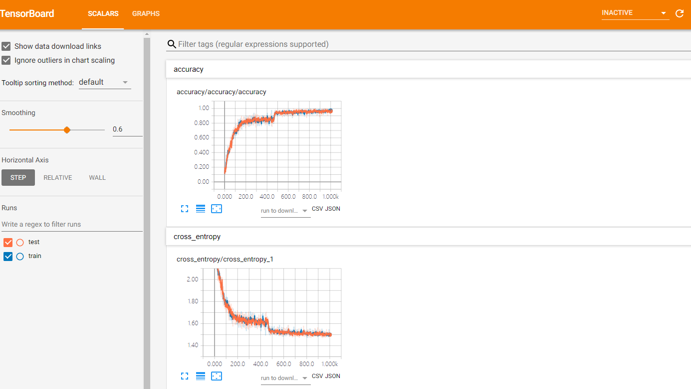
就可以进入tensorboard查看参数的可视化信息：