DCNN models
r
- RNN
- Fast RCNN
- Faster RCNN
- F-RCN
Faster RCNN
the first five layers is same as the ZF network.

the size of the input image is 224*224*3, after the first convolutional layer, the size of the feature map is 110*110*96( because the convolutional kernel is 7*7*3*96, 7,7 is width, and height of the kernel, 3 is the channels of the input, and 96 is the channels of the output. In caffe framework, all data is represent by blob, which is w*h*c*d, 110=(224-7+pad)/stride+1. The size of the first pooling layer is 3*3. the size of the feature map by the pooling layer is 55*55*96 ..... ) Finally, the model extract the output of the conv5(13*13*256), this feature map will be server as the input of the RPN.
RPN(region proposal network)
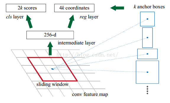
In the paper, 3*3 sliding windows is chosen. a 3*3*256*256 convolutional kernel is chosen to produce 256-d vectors(the size of the output is ((3-3)+1)*((3-3)+1)*256). between the cls layer and the 256-d layer, a 1*1*256*18 convolutional kernel is used, which is served as a fully connected layer. (if the size of the kernel is same as the input, it is called fully connected layer), For the reg layer, a 1*1*256*36 kernel is used. the network defined in caffe is:

- F-RCN: (region-based fully convolutional network)
F-RCN is faster than Faster RCNN, because the layers follow the ROI Pooling the connected layers. In F-RCN, there is not convolutional layer or fully connnected layers. and it use ResNet to take the place of ZF. In ResNet, most layers is convolutional layers. there are not pooling and fully connected layer, so it is categoried to fully convolutional network.
the intuition of the F-RCN is trying to speed up the Fast RCNN and share the calculation. F-RCN uses the first 100 layers of ResNet to extract feature map. The channels of the feature map is 2048, For reducing the dimension, a 1*1*2048*1024 kernel is added. and a convolutional layer is added to produce score maps for classification; and a convolutional layer is added to produce bounding box regression.
这个vote操作就是一个均值操作.

除了主网络ResNet以外,还有RPN网络用于生成ROI(region proposal),因此在训练的时候,作者采用RPN网络和R-FCN交替训练的方式来共享特征。
这里有个细节,假设每个image有N个ROI,那么在前向训练的时候会计算所有N个ROI的loss,然后将这N个ROI(包括positive和negative)按照loss高低进行排序,最后在backpropagation阶段只将loss最高的B个ROI的loss回传。详细可以参考OHEM算法。
因此为了将平移敏感性引入全卷积网络,作者在全卷积网络的输出位置添加一系列特定的卷积层用于生成position-sensitive的score map,每个score map保存目标的空间位置信息。然后再添加ROI Pooling层,该层后面不再跟卷积层或全连接层。这样整个网络不仅可以end-to-end训练,而且所有层的计算都是在整个图像上共享的。
如下图的table1,表示几种算法的共享层数情况。
Caffe的代码: 首先是数据读入操作,假设输出的data是1*3*600*1000,im_info是1*3,gt_boxes是1*4,后面的所有维度都是以这个假设为前提。

然后ResNet,结构如下图。R-FCN主要是采用ResNet和RPN结构来训练。R-FCN的具体结构(以ResNet50为例):conv1,maxpooling,conv2_x(在代码中用res2a_branch2a到res2c_branch2c表示,前面的字母a,b,c表示在conv2_x层需要循环3个大层,后面的a,b,c表示每个大层里面都有三个小层。另外还有res2a_branch1表示用1*1的256个卷积核卷积的结果。每个大层结束的时候都需要用Eltwise层合并,比如res2a_branch1和res2a_branch2c生成res2a,下一个大层则是res2a和res2b_branch2c座Eltwise合并),conv3_x,conv4_x,conv5_x。

然后是RPN网络,RPN网络以一个3*3的卷积核,pad=1,stride=1的512个卷积核的卷积层开始,输入是res4f层的输出,res4f层的输出即conv4_x最后的输出。该rpn_conv/3*3层的输出是1*512*38*63。

然后是分类层和回归层,分类层采用1*1的卷积核,pad=0,stride=1的18(2(back ground/fore ground)*9(anchors))个卷积核的卷积层,分类层的输出是1*18*38*63。回归采用1*1的卷积核,pad=0,stride=1的36(4*9(anchors))个卷积核的卷积层,回归层的输出是1*36*38*63。

Reshape层对分类层的结果做了一次维度调整,从1*18*38*63变成1*2*342*63,后面的342*63就代表该层所有anchor的数量。

下面这个层是用来从最开始读取的数据得到label和target。这里rpn_cls_score为1*1*342*63,rpn_bbox_targets为1*36*38*63,rpn_bbox_inside_weights为1*36*38*63,rpn_bbox_outside_weights为1*36*38*63。

损失函数如下:分类的损失采用SoftmaxWithLoss,输入是reshape后的预测的类别score(1*2*342*63)和真实的label(1*1*342*63)。回归的损失采用SmoothL1Loss,输入是rpn_bbox_pred(1*36*38*63)即所有anchor的坐标相关的预测,rpn_bbox_targets(1*36*38*63),rpn_bbox_inside_weights(1*36*38*63),rpn_bbox_outside_weights(1*36*38*63)。

然后是ROI Proposal,先用一个softmax层算出概率(1*2*342*63),然后再reshape到1*18*38*63。

然后是生成proposal,维度是1*5。

这一层生成rois(1*5*1*1),labels(1*1*1*1),bbox_targets(1*8*1*1),bbox_inside_weights (1*8*1*1),bbox_outside_weights(1*8*1*1)。

至此RPN网络结束。
新的卷积层,其实就是在ResNet后面添加的卷积层,以res5c作为输入,用1*1的卷积核,pad=0的1024个卷积核的卷积层。得到1*1024*38*63。

然后再分别跟两个卷积层,卷积核的大小都是1,pad=0,一个用于分类,一个用于回归。分类层如下:1*1029*38*63,其中1029的含义在下图中也有解释,21是代表类别(VOC的20类加上背景1类),7是和ROI要划分成7*7的格子对应。

这个分类层的输出结果就是论文中的这个三维矩阵:

然后是回归层的输出:1*392*38*63,与分类层类似。

开始进入ROI pooling操作了,上面一层,有两个输入:rfcn_cls(1*1029*38*63)是预测的结果,rois(1*5*1*1)是ROI,生成1*21*7*7的结果。下面一层是均值池化,得到1*21*1*1(cls_score),就是论文中vote的过程。

所以上面这两个操作就是对应论文中的这个图:

同理,回归也是类似的操作:生成1*8*7*7和1*8*1*1(bbox_pred)的结果。

最后就是损失和计算准确率层:

可以看出在ROI Pooling层后就没有卷积层和全连接层了。
总结:R-FCN作为Faster RCNN的改进版,主要对原有的ROI Pooling层进行改进和移位,使得不会存在众多region proposal都得经过全连接层的情况,这样就加快了速度。另一方面改进是将原来的VGG16类型的主网络换成ResNet系列网络。而算法的另一部分RPN网络则和Faster RCNN基本差不多。总的来讲实验效果还是很不错的。Caffe的代码: 首先是数据读入操作,假设输出的data是1*3*600*1000,im_info是1*3,gt_boxes是1*4,后面的所有维度都是以这个假设为前提。
然后ResNet,结构如下图。R-FCN主要是采用ResNet和RPN结构来训练。R-FCN的具体结构(以ResNet50为例):conv1,maxpooling,conv2_x(在代码中用res2a_branch2a到res2c_branch2c表示,前面的字母a,b,c表示在conv2_x层需要循环3个大层,后面的a,b,c表示每个大层里面都有三个小层。另外还有res2a_branch1表示用1*1的256个卷积核卷积的结果。每个大层结束的时候都需要用Eltwise层合并,比如res2a_branch1和res2a_branch2c生成res2a,下一个大层则是res2a和res2b_branch2c座Eltwise合并),conv3_x,conv4_x,conv5_x。
然后是RPN网络,RPN网络以一个3*3的卷积核,pad=1,stride=1的512个卷积核的卷积层开始,输入是res4f层的输出,res4f层的输出即conv4_x最后的输出。该rpn_conv/3*3层的输出是1*512*38*63。
然后是分类层和回归层,分类层采用1*1的卷积核,pad=0,stride=1的18(2(back ground/fore ground)*9(anchors))个卷积核的卷积层,分类层的输出是1*18*38*63。回归采用1*1的卷积核,pad=0,stride=1的36(4*9(anchors))个卷积核的卷积层,回归层的输出是1*36*38*63。
Reshape层对分类层的结果做了一次维度调整,从1*18*38*63变成1*2*342*63,后面的342*63就代表该层所有anchor的数量。
下面这个层是用来从最开始读取的数据得到label和target。这里rpn_cls_score为1*1*342*63,rpn_bbox_targets为1*36*38*63,rpn_bbox_inside_weights为1*36*38*63,rpn_bbox_outside_weights为1*36*38*63。
损失函数如下:分类的损失采用SoftmaxWithLoss,输入是reshape后的预测的类别score(1*2*342*63)和真实的label(1*1*342*63)。回归的损失采用SmoothL1Loss,输入是rpn_bbox_pred(1*36*38*63)即所有anchor的坐标相关的预测,rpn_bbox_targets(1*36*38*63),rpn_bbox_inside_weights(1*36*38*63),rpn_bbox_outside_weights(1*36*38*63)。
然后是ROI Proposal,先用一个softmax层算出概率(1*2*342*63),然后再reshape到1*18*38*63。
然后是生成proposal,维度是1*5。
这一层生成rois(1*5*1*1),labels(1*1*1*1),bbox_targets(1*8*1*1),bbox_inside_weights (1*8*1*1),bbox_outside_weights(1*8*1*1)。
至此RPN网络结束。
新的卷积层,其实就是在ResNet后面添加的卷积层,以res5c作为输入,用1*1的卷积核,pad=0的1024个卷积核的卷积层。得到1*1024*38*63。
然后再分别跟两个卷积层,卷积核的大小都是1,pad=0,一个用于分类,一个用于回归。分类层如下:1*1029*38*63,其中1029的含义在下图中也有解释,21是代表类别(VOC的20类加上背景1类),7是和ROI要划分成7*7的格子对应。
这个分类层的输出结果就是论文中的这个三维矩阵:
然后是回归层的输出:1*392*38*63,与分类层类似。
开始进入ROI pooling操作了,上面一层,有两个输入:rfcn_cls(1*1029*38*63)是预测的结果,rois(1*5*1*1)是ROI,生成1*21*7*7的结果。下面一层是均值池化,得到1*21*1*1(cls_score),就是论文中vote的过程。
所以上面这两个操作就是对应论文中的这个图:
同理,回归也是类似的操作:生成1*8*7*7和1*8*1*1(bbox_pred)的结果。
最后就是损失和计算准确率层:
可以看出在ROI Pooling层后就没有卷积层和全连接层了。
总结:R-FCN作为Faster RCNN的改进版,主要对原有的ROI Pooling层进行改进和移位,使得不会存在众多region proposal都得经过全连接层的情况,这样就加快了速度。另一方面改进是将原来的VGG16类型的主网络换成ResNet系列网络。而算法的另一部分RPN网络则和Faster RCNN基本差不多。总的来讲实验效果还是很不错的。
regression based
- YOLO
- SSD
DCNN models的更多相关文章
- 笔记:基于DCNN的图像语义分割综述
写在前面:一篇魏云超博士的综述论文,完整题目为<基于DCNN的图像语义分割综述>,在这里选择性摘抄和理解,以加深自己印象,同时达到对近年来图像语义分割历史学习和了解的目的,博古才能通今!感 ...
- Django models对象的select_related方法(减少查询次数)
表结构 先创建一个新的app python manage.py startapp test01 在settings.py注册一下app INSTALLED_APPS = ( 'django.contr ...
- Django models 操作高级补充
Django models 操作高级补充 字段参数补充: 外键 约束取消 ..... ORM中原生SQL写法: raw connection extra
- Django models Form model_form 关系及区别
Django models Form model_form
- Django models .all .values .values_list 几种数据查询结果的对比
Django models .all .values .values_list 几种数据查询结果的对比
- django models进行数据库增删查改
在cmd 上运行 python manage.py shell 引入models的定义 from app.models import myclass ##先打这一行 ------这些是 ...
- Django基础,Day2 - 编写urls,views,models
编写views views:作为MVC中的C,接收用户的输入,调用数据库Model层和业务逻辑Model层,处理后将处理结果渲染到V层中去. polls/views.py: from django.h ...
- 【Django】--Models 和ORM以及admin配置
Models 数据库的配置 1 django默认支持sqlite,mysql, oracle,postgresql数据库 <1>sqlite django默认使用sqlite的数据库 ...
- 广义线性模型(Generalized Linear Models)
前面的文章已经介绍了一个回归和一个分类的例子.在逻辑回归模型中我们假设: 在分类问题中我们假设: 他们都是广义线性模型中的一个例子,在理解广义线性模型之前需要先理解指数分布族. 指数分布族(The E ...
随机推荐
- 原生NodeJs制作一个简易聊天室
准备工作 安装NodeJs环境 安装编译器Sublime 如果网速不理想,可以百度一下如何加快npm的速度~ 使用node搭建一个简单的网站后台 做完准备工作之后,新建文件夹chatroom,在cha ...
- jmeter创建高级测试计划
如果应用程序使用重写地址而不是使用cookie存储信息,需要做一些额外的工作去测试程序 为了正确的响应重写地址,jmeter 需要解析 从服务器获取html 并且检索会话ID, 1 合理利用pre-p ...
- 一名网工对Linux运维的一次经历
我是一名名副其实的网络工程师,驻场于某市数字化城乡管理指挥中心(简称数字城管),主要针对中大型网络系统,路由.交换机.存储.小型机等设备进行维护,主要工作职责主要分为两种: 对网络系统中的网络设备(路 ...
- Beyond Compare 4过期
试用期到期操作:找到beyond Compare 4文件夹下面的BCUnrar.dll,将其删掉或者重命名,再重新打开接着使用!
- golang的interface剖析
背景: golang的interface是一种satisfied式的.A类只要实现了IA interface定义的方法,A就satisfied了接口IA.更抽象一层,如果某些设计上需要一些更抽象的 ...
- 自学Linux Shell4.3-处理数据文件sort grep gzip tar
点击返回 自学Linux命令行与Shell脚本之路 4.3-处理数据文件sort grep gzip tar ls命令用于显示文件目录列表,和Windows系统下DOS命令dir类似.当执行ls命令时 ...
- 【BZOJ3193】[JLOI2013]地形生成(动态规划)
[BZOJ3193][JLOI2013]地形生成(动态规划) 题面 BZOJ 洛谷 题解 第一问不难,首先按照山的高度从大往小排序,这样子只需要抉择前面有几座山就好了.然而有高度相同的山.其实也不麻烦 ...
- module 'scipy.misc' has no attribute 'toimage',python
anaconda环境下: 错误:python 命令行运行出错:module 'scipy.misc' has no attribute 'toimage' 解决:打开Anaconda prompt,输 ...
- EXGCD 扩展欧几里得
推荐:https://www.zybuluo.com/samzhang/note/541890 扩展欧几里得,就是求出来ax+by=gcd(x,y)的x,y 为什么有解? 根据裴蜀定理,存在u,v使得 ...
- CF 681
我太水了...... 这是一场奇差无比的CF. A,看题意有困难,实际上还是很水的. B,枚举 1234567 和 123456 的个数,时间复杂度1e6以下 C,业界毒瘤模拟题.最TM坑的是还要输出 ...