影评文本分类

官网示例：https://www.tensorflow.org/tutorials/keras/basic_text_classification
主要步骤：

1.加载IMDB数据集
2.探索数据：了解数据格式、将整数转换为字词
3.准备数据
4.构建模型：隐藏单元、损失函数和优化器
5.创建验证集
6.训练模型
7.评估模型
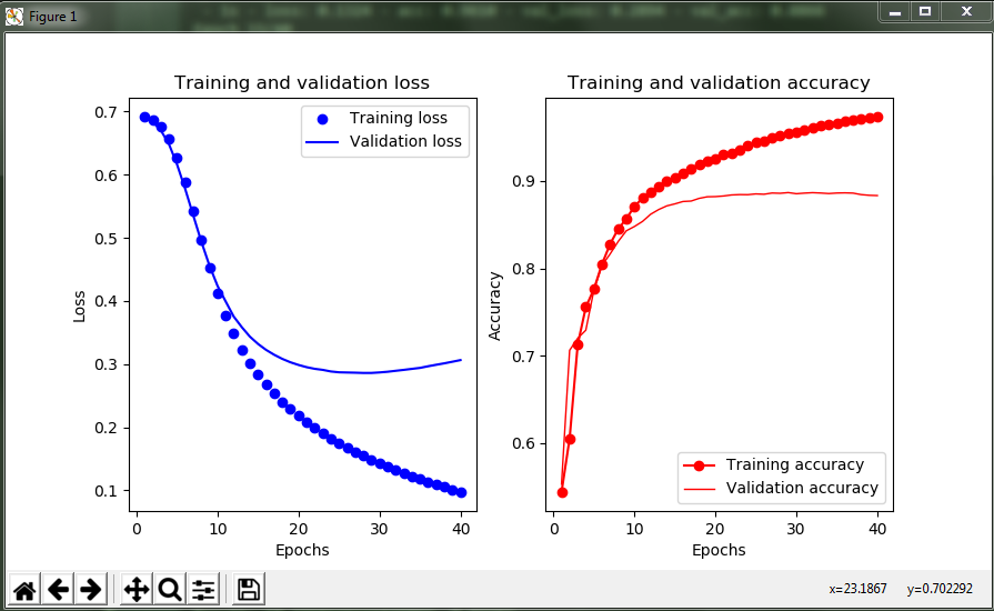
8.可视化：创建准确率和损失随时间变化的图

IMDB数据集

包含来自互联网电影数据库的50000条影评文本

MLCC文本分类指南

https://developers.google.com/machine-learning/guides/text-classification/

示例

脚本内容

GitHub：https://github.com/anliven/Hello-AI/blob/master/Google-Learn-and-use-ML/2_basic_text_classification.py

 # coding=utf-8

 import tensorflow as tf

 from tensorflow import keras

 import numpy as np

 import matplotlib.pyplot as plt

 import pathlib

 import os

 os.environ['TF_CPP_MIN_LOG_LEVEL'] = ''

 print("TensorFlow version: {}  - tf.keras version: {}".format(tf.VERSION, tf.keras.__version__))  # 查看版本

 ds_path = str(pathlib.Path.cwd()) + "\\datasets\\imdb\\"  # 数据集路径

 # ### 查看numpy格式数据

 np_data = np.load(ds_path + "imdb.npz")

 print("np_data keys: ", list(np_data.keys()))  # 查看所有的键

 # print("np_data values: ", list(np_data.values()))  # 查看所有的值

 # print("np_data items: ", list(np_data.items()))  # 查看所有的item

 # ### 加载IMDB数据集

 imdb = keras.datasets.imdb

 (train_data, train_labels), (test_data, test_labels) = imdb.load_data(

     path=ds_path + "imdb.npz",

     num_words=10000  # 保留训练数据中出现频次在前10000位的字词

 )

 # ### 探索数据：了解数据格式

 # 数据集已经过预处理：每个样本都是一个整数数组，表示影评中的字词

 # 每个标签都是整数值 0 或 1，其中 0 表示负面影评，1 表示正面影评

 print("Training entries: {}, labels: {}".format(len(train_data), len(train_labels)))

 print("First record: {}".format(train_data[0]))  # 第一条影评(影评文本已转换为整数，其中每个整数都表示字典中的一个特定字词)

 print("Before len:{} len:{}".format(len(train_data[0]), len(train_data[1])))  # 影评的长度会有所不同

 # 将整数转换回字词

 word_index = imdb.get_word_index(ds_path + "imdb_word_index.json")  # 整数值与词汇的映射字典

 word_index = {k: (v + 3) for k, v in word_index.items()}

 word_index["<PAD>"] = 0

 word_index["<START>"] = 1

 word_index["<UNK>"] = 2  # unknown

 word_index["<UNUSED>"] = 3

 reverse_word_index = dict([(value, key) for (key, value) in word_index.items()])

 def decode_review(text):

     """查询包含整数到字符串映射的字典对象"""

     return ' '.join([reverse_word_index.get(i, '?') for i in text])

 print("The content of first record: ", decode_review(train_data[0]))  # 显示第1条影评的文本

 # ### 准备数据

 # 影评（整数数组）必须转换为张量，然后才能馈送到神经网络中，而且影评的长度必须相同

 # 采用方法：填充数组，使之都具有相同的长度，然后创建一个形状为 max_length * num_reviews 的整数张量

 train_data = keras.preprocessing.sequence.pad_sequences(train_data,

                                                         value=word_index["<PAD>"],

                                                         padding='post',

                                                         maxlen=256)  # 使用 pad_sequences 函数将长度标准化

 test_data = keras.preprocessing.sequence.pad_sequences(test_data,

                                                        value=word_index["<PAD>"],

                                                        padding='post',

                                                        maxlen=256)

 print("After - len: {} len: {}".format(len(train_data[0]), len(train_data[1])))  # 样本的影评长度都已相同

 print("First record: \n", train_data[0])  # 填充后的第1条影评

 # ### 构建模型

 # 本示例中，输入数据由字词-索引数组构成。要预测的标签是 0 或 1

 # 按顺序堆叠各个层以构建分类器（模型有多少层，每个层有多少个隐藏单元）

 vocab_size = 10000  # 输入形状（用于影评的词汇数）

 model = keras.Sequential()  # 创建一个Sequential模型，然后通过简单地使用.add()方法将各层添加到模型

 # Embedding层：在整数编码的词汇表中查找每个字词-索引的嵌入向量

 # 模型在接受训练时会学习这些向量，会向输出数组添加一个维度(batch, sequence, embedding)

 model.add(keras.layers.Embedding(vocab_size, 16))

 # GlobalAveragePooling1D 层通过对序列维度求平均值，针对每个样本返回一个长度固定的输出向量

 model.add(keras.layers.GlobalAveragePooling1D())

 # 长度固定的输出向量会传入一个全连接 (Dense) 层（包含 16 个隐藏单元）

 model.add(keras.layers.Dense(16, activation=tf.nn.relu))

 # 最后一层与单个输出节点密集连接。应用sigmoid激活函数后，结果是介于 0 到 1 之间的浮点值，表示概率或置信水平

 model.add(keras.layers.Dense(1, activation=tf.nn.sigmoid))

 model.summary()  # 打印出关于模型的简单描述

 # ### 损失函数和优化器

 # 模型在训练时需要一个损失函数和一个优化器

 # 有多种类型的损失函数，一般来说binary_crossentropy更适合处理概率问题，可测量概率分布之间的“差距”

 model.compile(optimizer=tf.train.AdamOptimizer(),  # 优化器

               loss='binary_crossentropy',  # 损失函数

               metrics=['accuracy'])  # 在训练和测试期间的模型评估标准

 # ### 创建验证集

 # 仅使用训练数据开发和调整模型，然后仅使用一次测试数据评估准确率

 # 从原始训练数据中分离出验证集，可用于检查模型处理从未见过的数据的准确率

 x_val = train_data[:10000]  # 从原始训练数据中分离出10000个样本，创建一个验证集

 partial_x_train = train_data[10000:]

 y_val = train_labels[:10000]  # 从原始训练数据中分离出10000个样本，创建一个验证集

 partial_y_train = train_labels[10000:]

 # ### 训练模型

 # 对partial_x_train和partial_y_train张量中的所有样本进行迭代

 # 在训练期间，监控模型在验证集(x_val, y_val)的10000个样本上的损失和准确率

 history = model.fit(partial_x_train,

                     partial_y_train,

                     epochs=40,  # 训练周期（训练模型迭代轮次）

                     batch_size=512,  # 批量大小（每次梯度更新的样本数）

                     validation_data=(x_val, y_val),  # 验证数据

                     verbose=2  # 日志显示模式：0为安静模式, 1为进度条（默认）, 2为每轮一行

                     )  # 返回一个history对象，包含一个字典，其中包括训练期间发生的所有情况

 # ### 评估模型

 # 在测试模式下返回模型的误差值和评估标准值

 results = model.evaluate(test_data, test_labels)  # 返回两个值：损失（表示误差的数字，越低越好）和准确率

 print("Result: {}".format(results))

 # ### 可视化

 history_dict = history.history  # model.fit方法返回一个History回调，它具有包含连续误差的列表和其他度量的history属性

 print("Keys: {}".format(history_dict.keys()))  # 4个条目，每个条目对应训练和验证期间的一个受监控指标

 loss = history.history['loss']

 validation_loss = history.history['val_loss']

 accuracy = history.history['acc']

 validation_accuracy = history.history['val_acc']

 epochs = range(1, len(accuracy) + 1)

 plt.subplot(121)  # 创建损失随时间变化的图，作为1行2列图形矩阵中的第1个subplot

 plt.plot(epochs, loss, 'bo', label='Training loss')  # 绘制图形， 参数“bo”表示蓝色圆点状（blue dot）

 plt.plot(epochs, validation_loss, 'b', label='Validation loss')  # 参数“b”表示蓝色线状（solid blue line）

 plt.title('Training and validation loss')  # 标题

 plt.xlabel('Epochs')  # x轴标签

 plt.ylabel('Loss')  # y轴标签

 plt.legend()  # 绘制图例

 plt.subplot(122)  # 创建准确率随时间变化的图

 plt.plot(epochs, accuracy, color='red', marker='o', label='Training accuracy')

 plt.plot(epochs, validation_accuracy, 'r', linewidth=1, label='Validation accuracy')

 plt.title('Training and validation accuracy')

 plt.xlabel('Epochs')

 plt.ylabel('Accuracy')

 plt.legend()

 plt.savefig("./outputs/sample-2-figure.png", dpi=200, format='png')

 plt.show()  # 显示图形

运行结果

TensorFlow version: 1.12.0

np_data keys:  ['x_test', 'x_train', 'y_train', 'y_test']

Training entries: 25000, labels: 25000

First record: [1, 14, 22, 16, 43, 530, 973, 1622, 1385, 65, 458, 4468, 66, 3941, 4, 173, 36, 256, 5, 25, 100, 43, 838, 112, 50, 670, 2, 9, 35, 480, 284, 5, 150, 4, 172, 112, 167, 2, 336, 385, 39, 4, 172, 4536, 1111, 17, 546, 38, 13, 447, 4, 192, 50, 16, 6, 147, 2025, 19, 14, 22, 4, 1920, 4613, 469, 4, 22, 71, 87, 12, 16, 43, 530, 38, 76, 15, 13, 1247, 4, 22, 17, 515, 17, 12, 16, 626, 18, 2, 5, 62, 386, 12, 8, 316, 8, 106, 5, 4, 2223, 5244, 16, 480, 66, 3785, 33, 4, 130, 12, 16, 38, 619, 5, 25, 124, 51, 36, 135, 48, 25, 1415, 33, 6, 22, 12, 215, 28, 77, 52, 5, 14, 407, 16, 82, 2, 8, 4, 107, 117, 5952, 15, 256, 4, 2, 7, 3766, 5, 723, 36, 71, 43, 530, 476, 26, 400, 317, 46, 7, 4, 2, 1029, 13, 104, 88, 4, 381, 15, 297, 98, 32, 2071, 56, 26, 141, 6, 194, 7486, 18, 4, 226, 22, 21, 134, 476, 26, 480, 5, 144, 30, 5535, 18, 51, 36, 28, 224, 92, 25, 104, 4, 226, 65, 16, 38, 1334, 88, 12, 16, 283, 5, 16, 4472, 113, 103, 32, 15, 16, 5345, 19, 178, 32]

Before len:218 len:189

The content of first record:  <START> this film was just brilliant casting location scenery story direction everyone's really suited the part they played and you could just imagine being there robert <UNK> is an amazing actor and now the same being director <UNK> father came from the same scottish island as myself so i loved the fact there was a real connection with this film the witty remarks throughout the film were great it was just brilliant so much that i bought the film as soon as it was released for <UNK> and would recommend it to everyone to watch and the fly fishing was amazing really cried at the end it was so sad and you know what they say if you cry at a film it must have been good and this definitely was also <UNK> to the two little boy's that played the <UNK> of norman and paul they were just brilliant children are often left out of the <UNK> list i think because the stars that play them all grown up are such a big profile for the whole film but these children are amazing and should be praised for what they have done don't you think the whole story was so lovely because it was true and was someone's life after all that was shared with us all

After - len: 256 len: 256

First record:

 [   1   14   22   16   43  530  973 1622 1385   65  458 4468   66 3941

    4  173   36  256    5   25  100   43  838  112   50  670    2    9

   35  480  284    5  150    4  172  112  167    2  336  385   39    4

  172 4536 1111   17  546   38   13  447    4  192   50   16    6  147

 2025   19   14   22    4 1920 4613  469    4   22   71   87   12   16

   43  530   38   76   15   13 1247    4   22   17  515   17   12   16

  626   18    2    5   62  386   12    8  316    8  106    5    4 2223

 5244   16  480   66 3785   33    4  130   12   16   38  619    5   25

  124   51   36  135   48   25 1415   33    6   22   12  215   28   77

   52    5   14  407   16   82    2    8    4  107  117 5952   15  256

    4    2    7 3766    5  723   36   71   43  530  476   26  400  317

   46    7    4    2 1029   13  104   88    4  381   15  297   98   32

 2071   56   26  141    6  194 7486   18    4  226   22   21  134  476

   26  480    5  144   30 5535   18   51   36   28  224   92   25  104

    4  226   65   16   38 1334   88   12   16  283    5   16 4472  113

  103   32   15   16 5345   19  178   32    0    0    0    0    0    0

    0    0    0    0    0    0    0    0    0    0    0    0    0    0

    0    0    0    0    0    0    0    0    0    0    0    0    0    0

    0    0    0    0]

_________________________________________________________________

Layer (type)                 Output Shape              Param #

=================================================================

embedding (Embedding)        (None, None, 16)          160000

_________________________________________________________________

global_average_pooling1d (Gl (None, 16)                0

_________________________________________________________________

dense (Dense)                (None, 16)                272

_________________________________________________________________

dense_1 (Dense)              (None, 1)                 17

=================================================================

Total params: 160,289

Trainable params: 160,289

Non-trainable params: 0

_________________________________________________________________

Model summary:

Train on 15000 samples, validate on 10000 samples

Epoch 1/40

 - 1s - loss: 0.6914 - acc: 0.5768 - val_loss: 0.6887 - val_acc: 0.6371

Epoch 2/40

 - 1s - loss: 0.6835 - acc: 0.7170 - val_loss: 0.6784 - val_acc: 0.7431

Epoch 3/40

 - 1s - loss: 0.6680 - acc: 0.7661 - val_loss: 0.6591 - val_acc: 0.7566

Epoch 4/40

 - 1s - loss: 0.6407 - acc: 0.7714 - val_loss: 0.6290 - val_acc: 0.7724

Epoch 5/40

 - 1s - loss: 0.6016 - acc: 0.8012 - val_loss: 0.5880 - val_acc: 0.7914

Epoch 6/40

 - 1s - loss: 0.5543 - acc: 0.8191 - val_loss: 0.5435 - val_acc: 0.8059

Epoch 7/40

 - 1s - loss: 0.5040 - acc: 0.8387 - val_loss: 0.4984 - val_acc: 0.8256

Epoch 8/40

 - 1s - loss: 0.4557 - acc: 0.8551 - val_loss: 0.4574 - val_acc: 0.8390

Epoch 9/40

 - 1s - loss: 0.4132 - acc: 0.8659 - val_loss: 0.4227 - val_acc: 0.8483

Epoch 10/40

 - 1s - loss: 0.3763 - acc: 0.8795 - val_loss: 0.3946 - val_acc: 0.8558

Epoch 11/40

 - 1s - loss: 0.3460 - acc: 0.8874 - val_loss: 0.3740 - val_acc: 0.8601

Epoch 12/40

 - 1s - loss: 0.3212 - acc: 0.8929 - val_loss: 0.3540 - val_acc: 0.8689

Epoch 13/40

 - 1s - loss: 0.2984 - acc: 0.8999 - val_loss: 0.3402 - val_acc: 0.8713

Epoch 14/40

 - 1s - loss: 0.2796 - acc: 0.9057 - val_loss: 0.3280 - val_acc: 0.8737

Epoch 15/40

 - 1s - loss: 0.2633 - acc: 0.9101 - val_loss: 0.3187 - val_acc: 0.8762

Epoch 16/40

 - 1s - loss: 0.2493 - acc: 0.9141 - val_loss: 0.3110 - val_acc: 0.8786

Epoch 17/40

 - 1s - loss: 0.2356 - acc: 0.9200 - val_loss: 0.3046 - val_acc: 0.8791

Epoch 18/40

 - 1s - loss: 0.2237 - acc: 0.9237 - val_loss: 0.2994 - val_acc: 0.8810

Epoch 19/40

 - 1s - loss: 0.2126 - acc: 0.9278 - val_loss: 0.2955 - val_acc: 0.8829

Epoch 20/40

 - 1s - loss: 0.2028 - acc: 0.9316 - val_loss: 0.2920 - val_acc: 0.8832

Epoch 21/40

 - 1s - loss: 0.1932 - acc: 0.9347 - val_loss: 0.2893 - val_acc: 0.8836

Epoch 22/40

 - 1s - loss: 0.1844 - acc: 0.9389 - val_loss: 0.2877 - val_acc: 0.8843

Epoch 23/40

 - 1s - loss: 0.1765 - acc: 0.9421 - val_loss: 0.2867 - val_acc: 0.8853

Epoch 24/40

 - 1s - loss: 0.1685 - acc: 0.9469 - val_loss: 0.2852 - val_acc: 0.8844

Epoch 25/40

 - 1s - loss: 0.1615 - acc: 0.9494 - val_loss: 0.2848 - val_acc: 0.8858

Epoch 26/40

 - 1s - loss: 0.1544 - acc: 0.9522 - val_loss: 0.2850 - val_acc: 0.8859

Epoch 27/40

 - 1s - loss: 0.1486 - acc: 0.9543 - val_loss: 0.2860 - val_acc: 0.8847

Epoch 28/40

 - 1s - loss: 0.1424 - acc: 0.9573 - val_loss: 0.2857 - val_acc: 0.8867

Epoch 29/40

 - 1s - loss: 0.1367 - acc: 0.9587 - val_loss: 0.2867 - val_acc: 0.8867

Epoch 30/40

 - 1s - loss: 0.1318 - acc: 0.9607 - val_loss: 0.2882 - val_acc: 0.8863

Epoch 31/40

 - 1s - loss: 0.1258 - acc: 0.9634 - val_loss: 0.2899 - val_acc: 0.8868

Epoch 32/40

 - 1s - loss: 0.1212 - acc: 0.9652 - val_loss: 0.2919 - val_acc: 0.8854

Epoch 33/40

 - 1s - loss: 0.1159 - acc: 0.9679 - val_loss: 0.2941 - val_acc: 0.8853

Epoch 34/40

 - 1s - loss: 0.1115 - acc: 0.9690 - val_loss: 0.2972 - val_acc: 0.8852

Epoch 35/40

 - 1s - loss: 0.1077 - acc: 0.9705 - val_loss: 0.2988 - val_acc: 0.8845

Epoch 36/40

 - 1s - loss: 0.1028 - acc: 0.9727 - val_loss: 0.3020 - val_acc: 0.8841

Epoch 37/40

 - 1s - loss: 0.0990 - acc: 0.9737 - val_loss: 0.3050 - val_acc: 0.8830

Epoch 38/40

 - 1s - loss: 0.0956 - acc: 0.9745 - val_loss: 0.3087 - val_acc: 0.8824

Epoch 39/40

 - 1s - loss: 0.0914 - acc: 0.9765 - val_loss: 0.3109 - val_acc: 0.8832

Epoch 40/40

 - 1s - loss: 0.0878 - acc: 0.9780 - val_loss: 0.3148 - val_acc: 0.8822

   32/25000 [..............................] - ETA: 0s

 3328/25000 [==>...........................] - ETA: 0s

 7296/25000 [=======>......................] - ETA: 0s

11072/25000 [============>.................] - ETA: 0s

14304/25000 [================>.............] - ETA: 0s

17888/25000 [====================>.........] - ETA: 0s

21760/25000 [=========================>....] - ETA: 0s

25000/25000 [==============================] - 0s 16us/step

Result: [0.33562567461490633, 0.87216]

Keys: dict_keys(['val_loss', 'val_acc', 'loss', 'acc'])

问题处理

问题1：执行imdb.load_data()失败

错误提示：
Downloading data from https://storage.googleapis.com/tensorflow/tf-keras-datasets/imdb.npz
.......
Exception: URL fetch failure on https://storage.googleapis.com/tensorflow/tf-keras-datasets/imdb.npz: None -- [WinError 10060] A connection attempt failed because the connected party did not properly respond after a period of time, or established connection failed because connected host has failed to respond

处理方法：

方法1：手工下载文件，导入数据时参数path使用绝对路径；
方法2：手工下载文件，并存放在“~/.keras/datasets”目录下对应的文件夹；

问题2：执行imdb.get_word_index()失败

错误提示：
Downloading data from https://storage.googleapis.com/tensorflow/tf-keras-datasets/imdb_word_index.json
......
Exception: URL fetch failure on https://storage.googleapis.com/tensorflow/tf-keras-datasets/imdb_word_index.json: None -- [WinError 10060] A connection attempt failed because the connected party did not properly respond after a period of time, or established connection failed because connected host has failed to respond