Pytorch中RoI pooling layer的几种实现

Faster-RCNN论文中在RoI-Head网络中，将128个RoI区域对应的feature map进行截取，而后利用RoI pooling层输出7*7大小的feature map。在pytorch中可以利用：

• torch.nn.functional.adaptive_max_pool2d(input, output_size, return_indices=False)

• torch.nn.AdaptiveMaxPool2d(output_size, return_indices=False)

这个函数很方便调用，但是这个实现有个缺点，就是慢。

所以有许多其他不同的实现方式，借鉴其他人的实现方法，这里借鉴github做一个更加丰富对比实验。总共有4种方法：

方法1. 利用cffi进行C扩展实现,然后利用Pytorch调用：需要单独的 C 和 CUDA 源文件，还需要事先进行编译，不但过程比较繁琐，代码结构也稍显凌乱。对于一些简单的 CUDA 扩展（代码量不大，没有复杂的库依赖），显得不够友好。

方法2.利用Cupy实现在线编译，直接为 pytorch 提供 CUDA 扩展（当然，也可以是纯 C 的扩展）。Cupy实现了在cuda上兼容numpy格式的多维数组。GPU加速的矩阵运算，而Numpy并没有利用GPU。Cupy目前已脱离chainer成为一个独立的库。

方法3.利用chainer实现，相较其他深度学习框架来说，chainer知名度不够高，但是是一款非常优秀的深度学习框架，纯python实现，设计思想简洁，语法简单。chainer中的GPU加速也是通过Cupy实现的。此外，chainer还有其他附加包，例如ChainerCV，其中便有对Faster-RCNN、SSD等网络的实现。

  

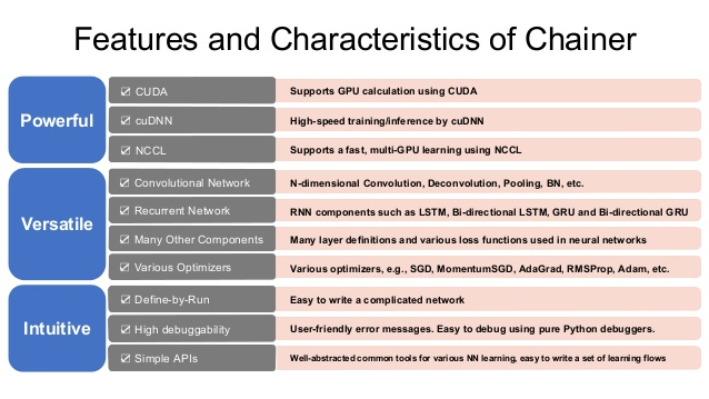
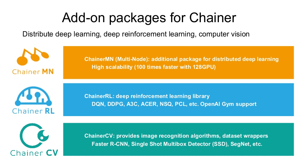
图源：Chainer官网slides

方法4.利用Pytorch实现，也就是文章伊始给出的两个函数。

从方法1至方法4，实现过程越来越简单，所以速度越来越慢。

以下是一个简单的对比试验结果：实验中以输入batch大小、图像尺寸（严格讲是特征图尺寸）大小、rois数目、是否反向传播为变量来进行对比，注意输出尺寸和Faster原论文一致都是7*7，都利用cuda，且设置scale=1，即特征图和原图同大小。

对比1： 只正向传播

use_cuda: True, has_backward: True
method1: 0.001353292465209961, batch_size: , size: , num_rois:
method2: 0.04485161781311035, batch_size: , size: , num_rois:
method3: 0.06167919635772705, batch_size: , size: , num_rois:
method4: 0.009436330795288085, batch_size: , size: , num_rois: 

method1: 0.0003777980804443359, batch_size: , size: , num_rois:
method2: 0.001593632698059082, batch_size: , size: , num_rois:
method3: 0.00210268497467041, batch_size: , size: , num_rois:
method4: 0.061138014793396, batch_size: , size: , num_rois: 

method1: 0.001754002571105957, batch_size: , size: , num_rois:
method2: 0.0047376775741577145, batch_size: , size: , num_rois:
method3: 0.006129913330078125, batch_size: , size: , num_rois:
method4: 0.06233139038085937, batch_size: , size: , num_rois: 

method1: 0.0018497371673583984, batch_size: , size: , num_rois:
method2: 0.010891580581665039, batch_size: , size: , num_rois:
method3: 0.023005642890930177, batch_size: , size: , num_rois:
method4: 0.5292188739776611, batch_size: , size: , num_rois: 

method1: 0.09110891819000244, batch_size: , size: , num_rois:
method2: 0.4102628231048584, batch_size: , size: , num_rois:
method3: 0.3902537250518799, batch_size: , size: , num_rois:
method4: 0.6544218873977661, batch_size: , size: , num_rois: 

method1: 0.09256606578826904, batch_size: , size: , num_rois:
method2: 0.641594967842102, batch_size: , size: , num_rois:
method3: 1.3756087446212768, batch_size: , size: , num_rois:
method4: 4.076273036003113, batch_size: , size: , num_rois: 

对比2：含反向传播

use_cuda: True, has_backward: False
method1: 0.000156359672546386, batch_size: , size: , num_rois:
method2: 0.009024391174316406, batch_size: , size: , num_rois:
method3: 0.009477467536926269, batch_size: , size: , num_rois:
method4: 0.002876405715942383, batch_size: , size: , num_rois: 

method1: 0.00017533779144287, batch_size: , size: , num_rois:
method2: 0.00040388107299804, batch_size: , size: , num_rois:
method3: 0.00085462093353271, batch_size: , size: , num_rois:
method4: 0.02638674259185791, batch_size: , size: , num_rois: 

method1: 0.00018683433532714, batch_size: , size: , num_rois:
method2: 0.00039398193359375, batch_size: , size: , num_rois:
method3: 0.00234550476074218, batch_size: , size: , num_rois:
method4: 0.02483976364135742, batch_size: , size: , num_rois: 

method1: 0.0013917160034179, batch_size: , size: , num_rois:
method2: 0.0010843658447265, batch_size: , size: , num_rois:
method3: 0.0025740385055541, batch_size: , size: , num_rois:
method4: 0.2577446269989014, batch_size: , size: , num_rois: 

method1: 0.0003826856613153, batch_size: , size: , num_rois:
method2: 0.0004550600051874, batch_size: , size: , num_rois:
method3: 0.2729876136779785, batch_size: , size: , num_rois:
method4: 0.0269237756729125, batch_size: , size: , num_rois: 

method1: 0.0008277797698974, batch_size: , size: , num_rois:
method2: 0.0021707582473754, batch_size: , size: , num_rois:
method3: 0.2724076747894287, batch_size: , size: , num_rois:
method4: 0.2687232542037964, batch_size: , size: , num_rois: 

可以观察到最后一种方法总是最慢的，因为对于所有的num_roi依次循环迭代，效率极低。

对比3：固定1个batch（一张图），size假设为50*50（特征图大小，所以原图为800*800），特征图通道设为512，num_rois设为300，这是近似于 batch为1的Faster-RCNN的测试过程，看一下用时情况：此时输入特征图为（1,512,50,50），rois为（300,5）。rois的第一列为batch index，因为是1个batch，所以此项全为0，没有实质作用。

use_cuda: True, has_backward: True
method0: 0.0344547653198242, batch_size: , size: , num_rois:
method1: 0.1322056961059570, batch_size: , size: , num_rois:
method2: 0.1307379817962646, batch_size: , size: , num_rois:
method3: 0.2016681671142578, batch_size: , size: , num_rois: 

可以看到，方法2和方法3速度几乎一致，所以可以使用更简洁的chainer方法，然而当使用多batch训练Faster时，最好利用方法1，速度极快。

代码已上传：github