Pytorch从0开始实现YOLO V3指南 part3——实现网络前向传播

本节翻译自：https://blog.paperspace.com/how-to-implement-a-yolo-v3-object-detector-from-scratch-in-pytorch-part-3/

前一节我们实现了YOLO结构中不同类型的层，这一节我们将用Pytorch来实现整个YOLO结构，定义网络的前向传播过程，最终能够实现给定一张图片获得检测输出。

这个项目使用python 3.5与Pytorch 0.4进行编写，官方地址。

必备条件：

1. 本教程的part1与part2
2. Pytorch的基本知识，包括如何使用nn.Module，nn.Sequential，torch.nn.parameter类构建常规的结构
3. 使用Pytorch处理图像

定义网络：

下面来为我们的检测器定义网络。在darknet.py文件中，我们增加下面的类。

class Darknet(nn.Module):
    def __init__(self, cfgfile):
        super(Darknet, self).__init__()
        self.blocks = parse_cfg(cfgfile)
        self.net_info, self.module_list = create_modules(self.blocks)

这里的类Darknet继承自nn.Modulel类。我们初始化类成员变量blocks,net_info和module_list。

实现网络前向传播：

网络的前向传播是采用复写nn.Module类的forward方法来实现的。

forward函数有两个目的，首先是计算输出，第二个就是将输出的检测特征图转换成能够轻松处理的格式（例如对它们进行变换使得跨多个比例的检测图能够连接在一起，因为它们的维度不同，不经转换无法连接）。

def forward(self, x, CUDA):
    modules = self.blocks[1:]
    outputs = {}   #We cache the outputs for the route layer

forward接受三个参数self、input x和CUDA，如果为CUDA真，将使用GPU加速前向过程。

我们从self.blocks[1:]开始迭代，这是因为self.blocks的第一个元素是net块，不是前向传播的内容。

Route和Shortcut层需要来自之前层的输出图，现在我们通过字典outputs缓存每一层的输出特征图，字典的键就是层的索引，值为特征图。

与create_modules函数一样，遍历包含网络模块的module_list。这里需要注意的是，模块的添加顺序与配置文件相同。这表示我们可以简单地传过每个模块来获得输出。

write = 0     #This is explained a bit later
for i, module in enumerate(modules):
    module_type = (module["type"])

Convolutional 和 Upsample 层：

如果模块为卷积模块或者是上采样模块，前传直接写成：

if module_type == "convolutional" or module_type == "upsample":
            x = self.module_list[i](x)

Route / Shortcut 层：

route的代码分为两种情况（见part2）。对于连接两个特征图这种情况我们使用torch.cat函数，第二个参数为1。这是因为我们希望在深度维上进行拼接（对于Pytorch来说维度为B*C*H*W，所以深度对应着第1维）。

 elif module_type == "route":
      layers = module["layers"]
      layers = [int(a) for a in layers]

      if (layers[0]) > 0:
           layers[0] = layers[0] - i

      if len(layers) == 1:
           x = outputs[i + (layers[0])]

      else:
          if (layers[1]) > 0:
             layers[1] = layers[1] - i

          map1 = outputs[i + layers[0]]
          map2 = outputs[i + layers[1]]

          x = torch.cat((map1, map2), 1)

 elif  module_type == "shortcut":
          from_ = int(module["from"])
          x = outputs[i-1] + outputs[i+from_]

YOLO(检测层)：

YOLO的输出是一个卷积特征图，特征图的深度方向是边界框的属性，cell预测的边界框属性彼此堆叠。因此，如果你要访问(5,6)处cell的第二个边界框，则必须通过map[5,6,(5+C):2*(5+C)] 来找到值。这种形式对于输出处理非常不方便，如对象置信度阈值化、向中心坐标添加网格偏移量、应用锚点等。

另一个问题是由于我们在三种尺度上做检测，预测图的维度将会不同。虽然这三个feature map的维度不同，但是要对它们执行的输出处理操作是相似的。最好是在一个张量上做这些运算，而不是在三个张量上。为了解决这些问题，我们引入了函数predict_transform。

 

转换输出：

predict_transform函数在util.py文件中，我们将其导入进来在Darknet类的前向传播中使用。

在util.py的前面导入必要的库

from __future__ import division

import torch
import torch.nn as nn
import torch.nn.functional as F
from torch.autograd import Variable
import numpy as np
import cv2 

predict_transform接收五个参数；prediction(我们的输出)，inp_dim(输入图片维度)，anchors, num_classes 和 CUDA标志位。

def predict_transform(prediction, inp_dim, anchors, num_classes, CUDA = True):

predict_transform函数接收一个检测的特征映射将其转换为一个2维的tensor，这里每行的tensor对应到一个边界框的属性，以如下形式：

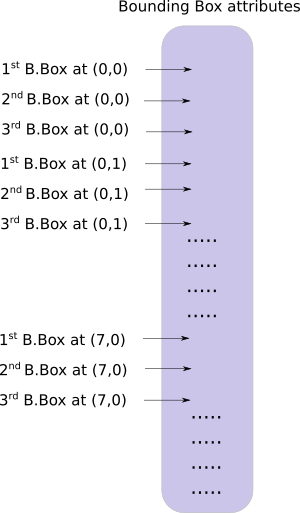
以下的代码来做上面的转换。

 batch_size = prediction.size(0)
 stride =  inp_dim // prediction.size(2)
 grid_size = inp_dim // stride
 bbox_attrs = 5 + num_classes
 num_anchors = len(anchors)

 prediction = prediction.view(batch_size, bbox_attrs*num_anchors, grid_size*grid_size)
 prediction = prediction.transpose(1,2).contiguous()
 prediction = prediction.view(batch_size, grid_size*grid_size*num_anchors, bbox_attrs)

锚的尺寸与net块的高度与宽度一致（使用的是[10,13] , [16,30], [33,23],这个的单位其实就是图片真实像素值），因此我们必须将锚除以检测特征图的步长。

anchors = [(a[0]/stride, a[1]/stride) for a in anchors]

现在，我们需要像Part1中讨论的那样转换我们的输出。

对x,y坐标与目标置信度进行sigmoid。

#Sigmoid the  centre_X, centre_Y. and object confidencce
prediction[:,:,0] = torch.sigmoid(prediction[:,:,0])
prediction[:,:,1] = torch.sigmoid(prediction[:,:,1])
prediction[:,:,4] = torch.sigmoid(prediction[:,:,4])

对中心坐标预测添加网格偏移。

#Add the center offsets
grid = np.arange(grid_size)
a,b = np.meshgrid(grid, grid)

x_offset = torch.FloatTensor(a).view(-1,1)
y_offset = torch.FloatTensor(b).view(-1,1)

if CUDA:
   x_offset = x_offset.cuda()
   y_offset = y_offset.cuda()

x_y_offset = torch.cat((x_offset, y_offset), 1).repeat(1,num_anchors).view(-1,2).unsqueeze(0)
prediction[:,:,:2] += x_y_offset

将锚点应用到包围框的维度上。

#log space transform height and the width
anchors = torch.FloatTensor(anchors)

if CUDA:
   anchors = anchors.cuda()

anchors = anchors.repeat(grid_size*grid_size, 1).unsqueeze(0)
prediction[:,:,2:4] = torch.exp(prediction[:,:,2:4])*anchors

在类得分上施加sigmoid激活函数。

prediction[:,:,5: 5 + num_classes] = torch.sigmoid((prediction[:,:, 5 : 5 + num_classes]))

最后一步，是将检测图放大到输入图片相同的尺寸。这里的边界框属性是根据特征图调整大小的。如果输入图片是416*416，特征图是13*13，我们就是将这些属性乘以步长也就是32.

prediction[:,:,:4] *= stride

这就是全部循环体的内容，在函数的结尾返回预测。

return prediction

Detection层回顾：

现在我们已经对输出向量进行了转换，能将三个不同尺寸下的检测图拼接组成一个大tensor。转换之前是做不到这点的，因为我们不能将拥有不同空间维的特征图拼接在一起。但现在我们的输出向量就像一个表格一样，以边界框作为它的行拼接起来就简单了。

我们在编程上遇到的一个障碍是不能初始化一个空向量，然后将它与一个非空向量拼接在一起。所以我们等到获得了第一张检测图后才初始化collector（保存检测的tensor），然后获得后续检测时才将特征映射拼接在一起。

注意write=0的标志位位于forward函数循环体之前。write标志位指明了我们是否获得了第一张检测图，write=0也就意味着还没有获得第一张检测图,当它为1的时候代表collector已经被初始化可以直接拼接检测图。

现在我们已经实现了predict_transform函数,下面在forward函数中编写处理检测特征图的代码。

在darknet.py的顶部，增加如下导入

from util import * 

之后在forward函数内部

 elif module_type == 'yolo':        

 　　anchors = self.module_list[i][0].anchors
 　　#Get the input dimensions
 　　inp_dim = int (self.net_info["height"])

 　　#Get the number of classes
 　　num_classes = int (module["classes"])

 　　#Transform
 　　x = x.data
 　　x = predict_transform(x, inp_dim, anchors, num_classes, CUDA)
 　　if not write:              #if no collector has been intialised.
       detections = x
       write = 1

 　　else:
        detections = torch.cat((detections, x), 1)

outputs[i] = x

最后返回检测结果

  return detections

测试前向传播过程：

这里有个创建虚拟输入的函数，我们将把这个输入到我们的网络。在写这个函数之前先将下面这张图片保存到你的工作路径。如果你是Linux用户，请输入：

wget https://github.com/ayooshkathuria/pytorch-yolo-v3/raw/master/dog-cycle-car.png

在darknet.py的前面定义下面这个函数：

def get_test_input():
    img = cv2.imread("dog-cycle-car.png")
    img = cv2.resize(img, (416,416))          #Resize to the input dimension
    img_ =  img[:,:,::-1].transpose((2,0,1))  # BGR -> RGB | H X W C -> C X H X W
    img_ = img_[np.newaxis,:,:,:]/255.0       #Add a channel at 0 (for batch) | Normalise
    img_ = torch.from_numpy(img_).float()     #Convert to float
    img_ = Variable(img_)                     # Convert to Variable
    return img_

接着输入以下代码：

model = Darknet("cfg/yolov3.cfg")
inp = get_test_input()
pred = model(inp, torch.cuda.is_available())
print (pred)

你会看到输出类似于：

(  0  ,.,.) =
   16.0962   17.0541   91.5104  ...     0.4336    0.4692    0.5279
   15.1363   15.2568  166.0840  ...     0.5561    0.5414    0.5318
   14.4763   18.5405  409.4371  ...     0.5908    0.5353    0.4979
               ⋱                ...
  411.2625  412.0660    9.0127  ...     0.5054    0.4662    0.5043
  412.1762  412.4936   16.0449  ...     0.4815    0.4979    0.4582
  412.1629  411.4338   34.9027  ...     0.4306    0.5462    0.4138
[torch.FloatTensor of size 1x10647x85]

这个tensor的维度为1*10647*85。第一维是批大小，因为我们只有一张图片所以是1。对于每张图片，我们都有10647*85的输出表格。表格的每一行代表了一个边界框（4个bbox属性，1个目标置信度，80个类得分）。

到目前为止，我们的网络都是随机的权重，所以不会产生正确的输出。下面我们将导入官方的权重文件。

下载预训练权重：

将预训练权重下载到你的检测器文件夹。可以点这里下载。如果你是Linux用户：

wget https://pjreddie.com/media/files/yolov3.weights

理解权重文件：

官方的权重文件是以串行方式存储的二进制文件。

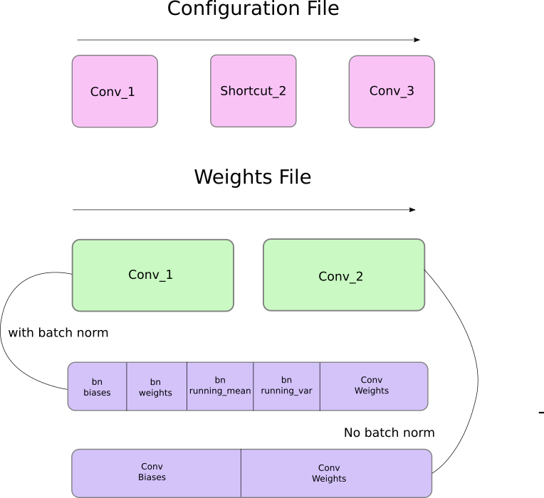
我们必须非常准确地加载权重。因为它仅仅作为浮点数存储，没有任何东西可以指导我们它属于哪个层，如果弄错了不会出现任何提示，比如说你可能把一个batch norm层的权值加载到卷积层了。因此，我们必须理解权重是如何存储的。

首先，权重只属于两种类型的层，要么是batch norm层，要么是卷积层。

这些层的权重完全按照它们在配置文件中出现的顺序存储。比如说一个卷积后面跟着一个Shortcut块，然后这个Shortcut块后面跟着另一个卷积块，权重文件也是先包含前一个卷积块的权重，然后是后一个卷积块的权重。

当batch norm层出现在卷积块中时，没有偏置参数。但是当没有batch norm层时，必须从文件中读取偏置的“权重”。

下图总结了权重是如何存储的。

 

加载权重

让我们来写程序加载权重吧！它作为Darknet类的成员函数。除了self之外还接收权重文件的路径。

def load_weights(self, weightfile):

开头的160个字节储存了5个int32的值，组成了文件头。

#Open the weights file
fp = open(weightfile, "rb")

#The first 5 values are header information
# 1. Major version number
# 2. Minor Version Number
# 3. Subversion number
# 4,5. Images seen by the network (during training)
header = np.fromfile(fp, dtype = np.int32, count = 5)
self.header = torch.from_numpy(header)
self.seen = self.header[3]

现在剩下的就代表权重了。权重是以float32或32-bit foat的形式存储的，现在使用一个np.ndarray加载剩下的权重。

weights = np.fromfile(fp, dtype = np.float32)

接着迭代权重文件，把它们加载到我们网络的模块中。

ptr = 0
for i in range(len(self.module_list)):
    module_type = self.blocks[i + 1]["type"]

    #If module_type is convolutional load weights
    #Otherwise ignore.

在循环体内部，我们先检查卷积块是否有batch_normalize。基于这个加载权重。

 if module_type == "convolutional":
     model = self.module_list[i]
     try:
          batch_normalize = int(self.blocks[i+1]["batch_normalize"])
     except:
          batch_normalize = 0

     conv = model[0]

我们保留一个名为ptr的变量来记录我们位于权重数组的位置。现在，如果batch_normalize为真，我们以如下方式加载权重。

if (batch_normalize):
      bn = model[1]

      #Get the number of weights of Batch Norm Layer
      num_bn_biases = bn.bias.numel()

      #Load the weights
      bn_biases = torch.from_numpy(weights[ptr:ptr + num_bn_biases])
      ptr += num_bn_biases

      bn_weights = torch.from_numpy(weights[ptr: ptr + num_bn_biases])
      ptr  += num_bn_biases

      bn_running_mean = torch.from_numpy(weights[ptr: ptr + num_bn_biases])
      ptr  += num_bn_biases

      bn_running_var = torch.from_numpy(weights[ptr: ptr + num_bn_biases])
      ptr  += num_bn_biases

      #Cast the loaded weights into dims of model weights.
      bn_biases = bn_biases.view_as(bn.bias.data)
      bn_weights = bn_weights.view_as(bn.weight.data)
      bn_running_mean = bn_running_mean.view_as(bn.running_mean)
      bn_running_var = bn_running_var.view_as(bn.running_var)

      #Copy the data to model
      bn.bias.data.copy_(bn_biases)
      bn.weight.data.copy_(bn_weights)
      bn.running_mean.copy_(bn_running_mean)
      bn.running_var.copy_(bn_running_var)

如果batch_normalize非真，直接加载卷积层的偏置

else:
     #Number of biases
     num_biases = conv.bias.numel()

     #Load the weights
     conv_biases = torch.from_numpy(weights[ptr: ptr + num_biases])
     ptr = ptr + num_biases

     #reshape the loaded weights according to the dims of the model weights
     conv_biases = conv_biases.view_as(conv.bias.data)

     #Finally copy the data
     conv.bias.data.copy_(conv_biases)

最后加载卷积层的权重

#Let us load the weights for the Convolutional layers
num_weights = conv.weight.numel()

#Do the same as above for weights
conv_weights = torch.from_numpy(weights[ptr:ptr+num_weights])
ptr = ptr + num_weights

conv_weights = conv_weights.view_as(conv.weight.data)
conv.weight.data.copy_(conv_weights)

加载权重的函数就此完成，现在你可以调用Darknet对象里面的load_wights函数

model = Darknet("cfg/yolov3.cfg")
model.load_weights("yolov3.weights")

这一部分到此结束，通过构建模型加载权重，我们终于能够检测目标了。在下一部分，你会学习如何使用目标置信度与非极大值抑制来产生我们最后的检测集合。

Further Reading

1. PyTorch tutorial
2. Reading binary files with NumPy
3. nn.Module, nn.Parameter classes