《DSP using MATLAB》Problem 3.17

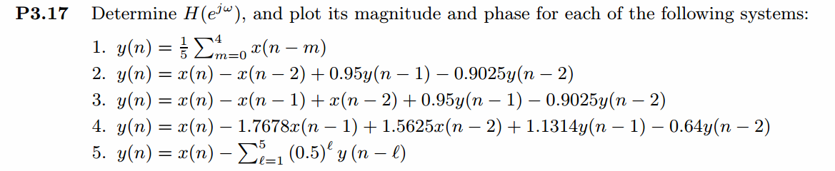
用差分方程两边进行z变换，再变量带换得到频率响应函数（或转移函数，即LTI系统脉冲响应的DTFT）。

代码：

%% ------------------------------------------------------------------------
%%            Output Info about this m-file
fprintf('\n***********************************************************\n');
fprintf('        <DSP using MATLAB> Problem 3.17 \n\n');

banner();
%% ------------------------------------------------------------------------

%% --------------------------------------------------------------
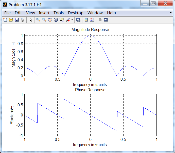
%%   1   y(n)=0.2*[x(n)+x(n-1)+x(n-2)+x(n-3)+x(n-4)]
%% --------------------------------------------------------------
a = [1];                                        % filter coefficient array a
b = [0.2, 0.2, 0.2, 0.2, 0.2];                  % filter coefficient array b

MM = 500;

H = freqresp1(b, a, MM);

magH  = abs(H);  angH  = angle(H);  realH  = real(H);  imagH  = imag(H);

%% --------------------------------------------------------------------
%%              START H's  mag ang real imag
%% --------------------------------------------------------------------
figure('NumberTitle', 'off', 'Name', 'Problem 3.17.1 H1');
set(gcf,'Color','white');
subplot(2,1,1); plot(w/pi,magH); grid on;  axis([-1,1,0,1.05]);
title('Magnitude Response');
xlabel('frequency in \pi units'); ylabel('Magnitude  |H|');
subplot(2,1,2); plot(w/pi, angH/pi); grid on;  axis([-1,1,-1.05,1.05]);
title('Phase Response');
xlabel('frequency in \pi units'); ylabel('Radians/\pi');

figure('NumberTitle', 'off', 'Name', 'Problem 3.17.1 H1');
set(gcf,'Color','white');
subplot(2,1,1); plot(w/pi, realH); grid on;
title('Real Part');
xlabel('frequency in \pi units'); ylabel('Real');
subplot(2,1,2); plot(w/pi, imagH); grid on;
title('Imaginary Part');
xlabel('frequency in \pi units'); ylabel('Imaginary');
%% -------------------------------------------------------------------
%%             END X's  mag ang real imag
%% -------------------------------------------------------------------

%% --------------------------------------------------------------
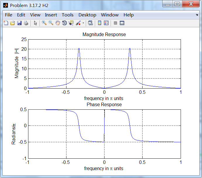
%%   2   y(n)=x(n)-x(n-2)+0.95y(n-1)-0.9025y(n-2)
%% --------------------------------------------------------------
a = [1, -0.95, 0.9025];                    % filter coefficient array a
b = [1, 0, -1];                            % filter coefficient array b

MM = 500;

H = freqresp1(b, a, MM);

magH  = abs(H);  angH  = angle(H);  realH  = real(H);  imagH  = imag(H);

%% --------------------------------------------------------------------
%%              START H's  mag ang real imag
%% --------------------------------------------------------------------
figure('NumberTitle', 'off', 'Name', 'Problem 3.17.2 H2');
set(gcf,'Color','white');
subplot(2,1,1); plot(w/pi,magH); grid on;  %axis([-1,1,0,1.05]);
title('Magnitude Response');
xlabel('frequency in \pi units'); ylabel('Magnitude  |H|');
subplot(2,1,2); plot(w/pi, angH/pi); grid on;  %axis([-1,1,-1.05,1.05]);
title('Phase Response');
xlabel('frequency in \pi units'); ylabel('Radians/\pi');

figure('NumberTitle', 'off', 'Name', 'Problem 3.17.2 H2');
set(gcf,'Color','white');
subplot(2,1,1); plot(w/pi, realH); grid on;
title('Real Part');
xlabel('frequency in \pi units'); ylabel('Real');
subplot(2,1,2); plot(w/pi, imagH); grid on;
title('Imaginary Part');
xlabel('frequency in \pi units'); ylabel('Imaginary');
%% -------------------------------------------------------------------
%%             END X's  mag ang real imag
%% -------------------------------------------------------------------

%% --------------------------------------------------------------
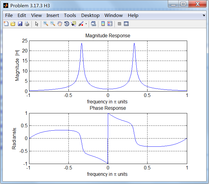
%%   3   y(n)=x(n)-x(n-1)-x(n-2)+0.95y(n-1)-0.9025y(n-2)
%% --------------------------------------------------------------
a = [1, -0.95, 0.9025];                    % filter coefficient array a
b = [1, -1, -1];                           % filter coefficient array b

MM = 500;
H = freqresp1(b, a, MM);

magH  = abs(H);  angH  = angle(H);  realH  = real(H);  imagH  = imag(H);

%% --------------------------------------------------------------------
%%              START H's  mag ang real imag
%% --------------------------------------------------------------------
figure('NumberTitle', 'off', 'Name', 'Problem 3.17.3 H3');
set(gcf,'Color','white');
subplot(2,1,1); plot(w/pi,magH); grid on;  %axis([-1,1,0,1.05]);
title('Magnitude Response');
xlabel('frequency in \pi units'); ylabel('Magnitude  |H|');
subplot(2,1,2); plot(w/pi, angH/pi); grid on;  %axis([-1,1,-1.05,1.05]);
title('Phase Response');
xlabel('frequency in \pi units'); ylabel('Radians/\pi');

figure('NumberTitle', 'off', 'Name', 'Problem 3.17.3 H3');
set(gcf,'Color','white');
subplot(2,1,1); plot(w/pi, realH); grid on;
title('Real Part');
xlabel('frequency in \pi units'); ylabel('Real');
subplot(2,1,2); plot(w/pi, imagH); grid on;
title('Imaginary Part');
xlabel('frequency in \pi units'); ylabel('Imaginary');
%% -------------------------------------------------------------------
%%             END X's  mag ang real imag
%% -------------------------------------------------------------------

%% --------------------------------------------------------------
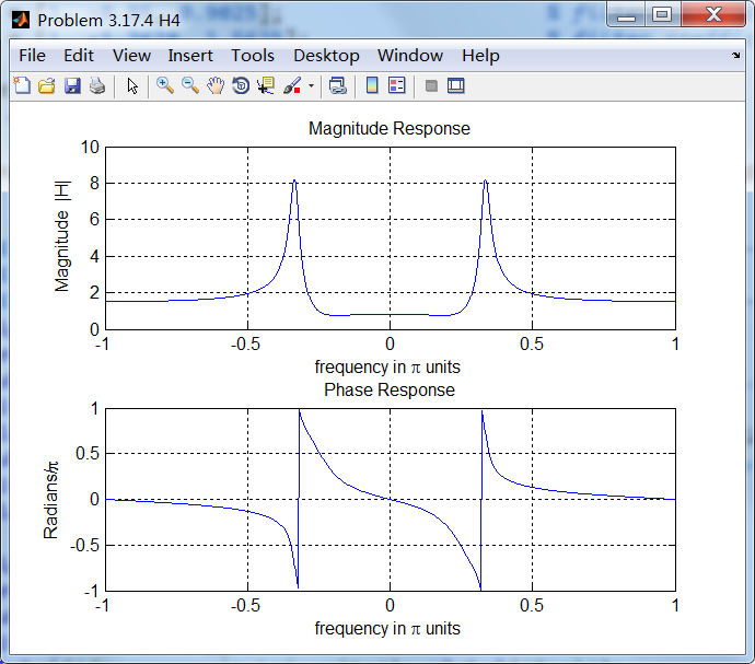
%%   4   y(n)=x(n)-1.7678x(n-1)+1.5625x(n-2)
%%               +0.95y(n-1)-0.9025y(n-2)
%% --------------------------------------------------------------
a = [1, -0.95, 0.9025];                    % filter coefficient array a
b = [1, -1.7678, 1.5625];                  % filter coefficient array b

MM = 500;
H = freqresp1(b, a, MM);

magH  = abs(H);  angH  = angle(H);  realH  = real(H);  imagH  = imag(H);

%% --------------------------------------------------------------------
%%              START H's  mag ang real imag
%% --------------------------------------------------------------------
figure('NumberTitle', 'off', 'Name', 'Problem 3.17.4 H4');
set(gcf,'Color','white');
subplot(2,1,1); plot(w/pi,magH); grid on;  %axis([-1,1,0,1.05]);
title('Magnitude Response');
xlabel('frequency in \pi units'); ylabel('Magnitude  |H|');
subplot(2,1,2); plot(w/pi, angH/pi); grid on;  %axis([-1,1,-1.05,1.05]);
title('Phase Response');
xlabel('frequency in \pi units'); ylabel('Radians/\pi');

figure('NumberTitle', 'off', 'Name', 'Problem 3.17.4 H4');
set(gcf,'Color','white');
subplot(2,1,1); plot(w/pi, realH); grid on;
title('Real Part');
xlabel('frequency in \pi units'); ylabel('Real');
subplot(2,1,2); plot(w/pi, imagH); grid on;
title('Imaginary Part');
xlabel('frequency in \pi units'); ylabel('Imaginary');
%% -------------------------------------------------------------------
%%             END X's  mag ang real imag
%% -------------------------------------------------------------------

%% ------------------------------------------------------------------------------
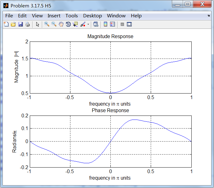
%%   5   y(n)=x(n)-0.5y(n-1)-0.25y(n-2)-0.125y(n-3)-0.0625y(n-4)-0.03125y(n-5)
%%
%% ------------------------------------------------------------------------------
a = [1, 0.5, 0.25, 0.125, 0.0625, 0.03125];         % filter coefficient array a
b = [1];                                            % filter coefficient array b

MM = 500;
H = freqresp1(b, a, MM);

magH  = abs(H);  angH  = angle(H);  realH  = real(H);  imagH  = imag(H);

%% --------------------------------------------------------------------
%%              START H's  mag ang real imag
%% --------------------------------------------------------------------
figure('NumberTitle', 'off', 'Name', 'Problem 3.17.5 H5');
set(gcf,'Color','white');
subplot(2,1,1); plot(w/pi,magH); grid on;  %axis([-1,1,0,1.05]);
title('Magnitude Response');
xlabel('frequency in \pi units'); ylabel('Magnitude  |H|');
subplot(2,1,2); plot(w/pi, angH/pi); grid on;  %axis([-1,1,-1.05,1.05]);
title('Phase Response');
xlabel('frequency in \pi units'); ylabel('Radians/\pi');

figure('NumberTitle', 'off', 'Name', 'Problem 3.17.5 H5');
set(gcf,'Color','white');
subplot(2,1,1); plot(w/pi, realH); grid on;
title('Real Part');
xlabel('frequency in \pi units'); ylabel('Real');
subplot(2,1,2); plot(w/pi, imagH); grid on;
title('Imaginary Part');
xlabel('frequency in \pi units'); ylabel('Imaginary');
%% -------------------------------------------------------------------
%%             END X's  mag ang real imag
%% -------------------------------------------------------------------

　　运行结果：