Deep Learning Tutorial - Convolutional Neural Networks(LENET)

CNN很多概述和要点在CS231n、Neural Networks and Deep Learning中有详细阐述，这里补充Deep Learning Tutorial中的内容。本节前提是前两节的内容，因为要用到全连接层、logistic regression层等。关于Theano：掌握共享变量，下采样，conv2d，dimshuffle的应用等。

1.卷积操作

在Theano中，ConvOp是提供卷积操作的主力。ConvOp来自theano.tensor.signal.conv.conv2d，有两个参数输入[input, W]：

1）input：对应于小批量输入图像的4维张量。尺寸为[小批量尺寸，特征映射数量（滤波器数量），图像高度，图像宽度]

2）W：对应于权重W的4维张量。尺寸为[第m层滤波器数量，m-1层滤波器数量，滤波器高度，滤波器宽度]

但是下面这段代码没有使用这个函数，而是另一个theano.tensor.nnet.conv2d，后面再做解释。

# coding=utf-8
import theano
from theano import tensor as T
from theano.tensor.nnet import conv
import numpy
import numpy
import pylab
from PIL import Image

rng = numpy.random.RandomState(23455)
input = T.tensor4(name='input')       #初始化4维张量类型！
w_shp = (2, 3, 9, 9)   #2个滤波器，3通道，9*9滤波窗口（感受野）
w_bound = numpy.sqrt(3 * 9 * 9)
W = theano.shared(numpy.asarray(rng.uniform(low=-1.0 / w_bound,high=1.0 / w_bound,size=w_shp),dtype=input.dtype), name ='W')
b_shp = (2,)
b = theano.shared(numpy.asarray(rng.uniform(low=-.5, high=.5, size=b_shp),dtype=input.dtype), name ='b')
conv_out = conv.conv2d(input, W)  #求卷积
output = T.nnet.sigmoid(conv_out + b.dimshuffle('x', 0, 'x', 'x'))
f = theano.function([input], output)    #卷积操作函数

img = Image.open('3wolfmoon.jpg')    #文档中给出的3狼图像（639，516，3）
img = numpy.asarray(img, dtype='float64') / 256.
img_ = img.transpose(2, 0, 1).reshape(1, 3, 639, 516)   #图像变形为（1,3,639,516）
filtered_img = f(img_)    #求卷积
pylab.subplot(1, 3, 1); pylab.axis('off'); pylab.imshow(img)
pylab.gray();
pylab.subplot(1, 3, 2); pylab.axis('off'); pylab.imshow(filtered_img[0, 0, :, :])   #第一滤波器结果
pylab.subplot(1, 3, 3); pylab.axis('off'); pylab.imshow(filtered_img[0, 1, :, :])   #第二滤波器结果
pylab.show()

代码结果：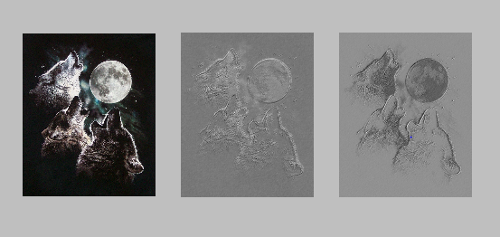

由图中可以看出，随机初始化形成的滤波器经过卷积操作类似于边缘描述子

2.池化（pooling）

Cnn的一个重要步骤是池化，是一种非线性的下采样。比较重要和常见的是最大值采样。在Theano中用 theano.tensor.signal.downsample.max_pool_2d来进行。输入为N维张量（tensor）N>2。下面有一个应用例子，分别是忽略边界和不忽略边界：

from theano.tensor.signal import downsample
input = T.dtensor4(’input’)
maxpool_shape = (2, 2)    #2*2的一个池化窗口
pool_out = downsample.max_pool_2d(input, maxpool_shape, ignore_border=True)       #忽略边界的池化
f = theano.function([input],pool_out)
invals = numpy.random.RandomState(1).rand(3, 2, 5, 5)
print ’With ignore_border set to True:’
print ’invals[0, 0, :, :] =\n’, invals[0, 0, :, :]
print ’output[0, 0, :, :] =\n’, f(invals)[0, 0, :, :]
pool_out = downsample.max_pool_2d(input, maxpool_shape, ignore_border=False)      #保留边界的池化
f = theano.function([input],pool_out)
print ’With ignore_border set to False:’
print ’invals[1, 0, :, :] =\n ’, invals[1, 0, :, :]
print ’output[1, 0, :, :] =\n ’, f(invals)[1, 0, :, :]

3.完整模型：LeNet

Sparse（稀疏连接），convolutional layers（卷积层）和max-pooling（最大值池化）是LeNet家族模型的核心。虽然细节差别很大，下图展示了LeNet几何模型：

上图结构很明了，（卷积+池化）*2+全连接层（MLP），这个全连接层是很传统的一种，包含隐层+logsitic regression，这俩前两节都有介绍。现在讨论theano.tensor.nnet.conv2d和theano.tensor.signal.conv.conv.2d.前者在目前几乎所有模型中使用最多，在这个操作中，每个输出的特征映射与输入的特征映射通过2维滤波器相联系，其值为通过对应滤波器进行卷积操作的和。在原始LeNet中，输出特征映射只与输入特征映射的子集有关系。那么后者只用在信号处理中。

4.主代码

# coding=UTF-8
from __future__ import print_function
import os
import sys
import timeit

import numpy

import theano
import theano.tensor as T
from theano.tensor.signal import pool
from theano.tensor.nnet import conv2d

from Logistic_sgd import LogisticRegression, load_data
from mlp import HiddenLayer

class LeNetConvPoolLayer(object):
    """Pool Layer of a convolutional network """
    def __init__(self, rng, input, filter_shape, image_shape, poolsize=(2, 2)):
        assert image_shape[1] == filter_shape[1]
        self.input = input
        # there are "num input feature maps * filter height * filter width"
        # inputs to each hidden unit
        fan_in = numpy.prod(filter_shape[1:])  # 维度拉成列，每个元素都为一个像素，fan_out同理
        # each unit in the lower layer receives a gradient from:
        # "num output feature maps * filter height * filter width" / pooling size
        fan_out = (filter_shape[0] * numpy.prod(filter_shape[2:]) /numpy.prod(poolsize))
        W_bound = numpy.sqrt(6. / (fan_in + fan_out))
        self.W = theano.shared(numpy.asarray(rng.uniform(low=-W_bound, high=W_bound, size=filter_shape),
                dtype=theano.config.floatX),borrow=True)
        b_values = numpy.zeros((filter_shape[0],), dtype=theano.config.floatX)
        self.b = theano.shared(value=b_values, borrow=True)

        conv_out = conv2d(     #利用滤波器进行卷积操作
            input=input,
            filters=self.W,
            filter_shape=filter_shape,
            input_shape=image_shape
        )

        pooled_out = pool.pool_2d(   #池化：最大值池化
            input=conv_out,
            ds=poolsize,
            ignore_border=True
        )
        self.output = T.tanh(pooled_out + self.b.dimshuffle('x', 0, 'x', 'x'))  #对阈值参数b维度进行调整
        self.params = [self.W, self.b]          #'x'看作1,0看作第零维度，这里调整后为b=(1,0维度,1,1)
        self.input = input                      #若b本身为(5,1)，则零维度为5，即b=(1,5,1,1)

def evaluate_lenet5(learning_rate=0.1, n_epochs=200,dataset='mnist.pkl.gz',nkerns=[20, 50], batch_size=500):
    rng = numpy.random.RandomState(23455)       #nkerns:两次卷积的滤波器个数本别为20，50
    datasets = load_data(dataset)
    train_set_x, train_set_y = datasets[0]
    valid_set_x, valid_set_y = datasets[1]
    test_set_x, test_set_y = datasets[2]

    n_train_batches = train_set_x.get_value(borrow=True).shape[0] / batch_size
    n_valid_batches = valid_set_x.get_value(borrow=True).shape[0] / batch_size
    n_test_batches = test_set_x.get_value(borrow=True).shape[0] / batch_size

    index = T.lscalar()
    x = T.matrix('x')
    y = T.ivector('y')
    print('... building the model')

    layer0_input = x.reshape((batch_size, 1, 28, 28))  #mnist数据集图片尺寸28*28

    # Construct the first convolutional pooling layer:
    # filtering reduces the image size to (28-5+1 , 28-5+1) = (24, 24)
    # maxpooling reduces this further to (24/2, 24/2) = (12, 12)
    # 4D output tensor is thus of shape (batch_size, nkerns[0], 12, 12)
    layer0 = LeNetConvPoolLayer(   #输入（batch_size,1,28,28）,输出（batch_size,20,12,12）
        rng,
        input=layer0_input,
        image_shape=(batch_size, 1, 28, 28),
        filter_shape=(nkerns[0], 1, 5, 5),   #滤波器个数，灰度图像通道数为1，5*5的感受野
        poolsize=(2, 2)
    )

    # Construct the second convolutional pooling layer
    # filtering reduces the image size to (12-5+1, 12-5+1) = (8, 8)
    # maxpooling reduces this further to (8/2, 8/2) = (4, 4)
    # 4D output tensor is thus of shape (batch_size, nkerns[1], 4, 4)
    layer1 = LeNetConvPoolLayer(   #输入（batch_size,20,12,12），输出（batch_size,1,4,4）
        rng,
        input=layer0.output,
        image_shape=(batch_size, nkerns[0], 12, 12),
        filter_shape=(nkerns[1], nkerns[0], 5, 5),
        poolsize=(2, 2)
    )

    # the HiddenLayer being fully-connected, it operates on 2D matrices of
    # shape (batch_size, num_pixels) (i.e matrix of rasterized images).
    # This will generate a matrix of shape (batch_size, nkerns[1] * 4 * 4),
    # or (500, 50 * 4 * 4) = (500, 800) with the default values.
    layer2_input = layer1.output.flatten(2)   # 因为要进入全连接层，拉成一维向量即50*4*4

    # construct a fully-connected sigmoidal layer
    layer2 = HiddenLayer(  #输入50*4*4，输出500
        rng,
        input=layer2_input,
        n_in=nkerns[1] * 4 * 4,
        n_out=500,
        activation=T.tanh
    )

    # classify the values of the fully-connected sigmoidal layer
    layer3 = LogisticRegression(input=layer2.output, n_in=500, n_out=10)  #输入500，输出10

    # the cost we minimize during training is the NLL of the model
    cost = layer3.negative_log_likelihood(y)

    # create a function to compute the mistakes that are made by the model
    test_model = theano.function(             #测试模型
        [index],
        layer3.errors(y),
        givens={
            x: test_set_x[index * batch_size: (index + 1) * batch_size],
            y: test_set_y[index * batch_size: (index + 1) * batch_size]
        }
    )

    validate_model = theano.function(         #验证模型
        [index],
        layer3.errors(y),
        givens={
            x: valid_set_x[index * batch_size: (index + 1) * batch_size],
            y: valid_set_y[index * batch_size: (index + 1) * batch_size]
        }
    )
    params = layer3.params + layer2.params + layer1.params + layer0.params  #参数集
    grads = T.grad(cost, params)   #求梯度
    updates = [(param_i, param_i - learning_rate * grad_i) for param_i, grad_i in zip(params, grads)]
    # 参数太多，寻找更新方式太冗长，所以利用SGD更新（来自翻译）
    train_model = theano.function(            #训练模型
        [index],
        cost,
        updates=updates,
        givens={
            x: train_set_x[index * batch_size: (index + 1) * batch_size],
            y: train_set_y[index * batch_size: (index + 1) * batch_size]
        }
    )
    print('... training')
    # early-stopping 策略
    patience = 10000  # look as this many examples regardless
    patience_increase = 2  # wait this much longer when a new best is found
    improvement_threshold = 0.995  # a relative improvement of this much is considered significant
    validation_frequency = min(n_train_batches, patience // 2)
    # go through this many minibatche before checking the network on the validation set; in this case we check every epoch
    best_validation_loss = numpy.inf
    best_iter = 0
    test_score = 0.
    start_time = timeit.default_timer()
    epoch = 0
    done_looping = False

    while (epoch < n_epochs) and (not done_looping):
        epoch = epoch + 1
        for minibatch_index in range(n_train_batches):

            iter = (epoch - 1) * n_train_batches + minibatch_index

            if iter % 100 == 0:
                print('training @ iter = ', iter)
            cost_ij = train_model(minibatch_index)

            if (iter + 1) % validation_frequency == 0:
                # compute zero-one loss on validation set
                validation_losses = [validate_model(i) for i in range(n_valid_batches)]
                this_validation_loss = numpy.mean(validation_losses)
                print('epoch %i, minibatch %i/%i, validation error %f %%' %(epoch, minibatch_index + 1, n_train_batches, this_validation_loss * 100.))

                # if we got the best validation score until now
                if this_validation_loss < best_validation_loss:
                    #improve patience if loss improvement is good enough
                    if this_validation_loss < best_validation_loss *  \
                       improvement_threshold:
                        patience = max(patience, iter * patience_increase)

                    # save best validation score and iteration number
                    best_validation_loss = this_validation_loss
                    best_iter = iter

                    # test it on the test set
                    test_losses = [test_model(i)for i in range(n_test_batches)]
                    test_score = numpy.mean(test_losses)
                    print(('epoch %i, minibatch %i/%i, test error of ''best model %f %%') %(epoch, minibatch_index + 1, n_train_batches, test_score * 100.))

            if patience <= iter:
                done_looping = True
                break

    end_time = timeit.default_timer()
    print('Optimization complete.')
    print('Best validation score of %f %% obtained at iteration %i, '
          'with test performance %f %%' %
          (best_validation_loss * 100., best_iter + 1, test_score * 100.))
    print(('The code for file ' +
           os.path.split(__file__)[1] +
           ' ran for %.2fm' % ((end_time - start_time) / 60.)), file=sys.stderr)

if __name__ == '__main__':
    evaluate_lenet5()

def experiment(state, channel):
    evaluate_lenet5(state.learning_rate, dataset=state.dataset)