PCA and Whitening on natural images

Step 0: Prepare data

Step 0a: Load data

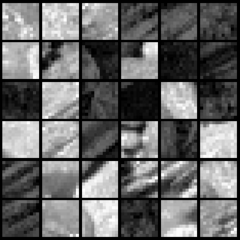
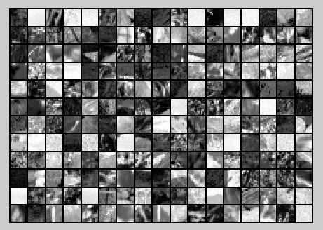
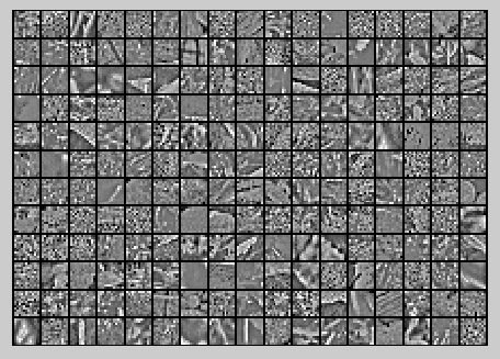
The starter code contains code to load a set of natural images and sample 12x12 patches from them. The raw patches will look something like this:

These patches are stored as column vectors in the matrix x.

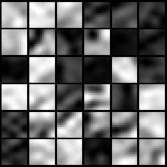
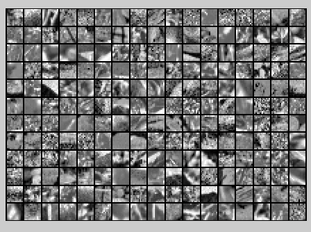
Step 0b: Zero mean the data

First, for each image patch, compute the mean pixel value and subtract it from that image, this centering the image around zero. You should compute a different mean value for each image patch.

Step 1: Implement PCA

Step 1a: Implement PCA

In this step, you will implement PCA to obtain x_rot, the matrix in which the data is "rotated" to the basis comprising the principal components

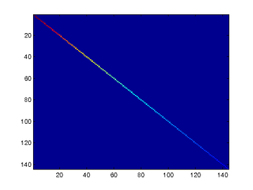
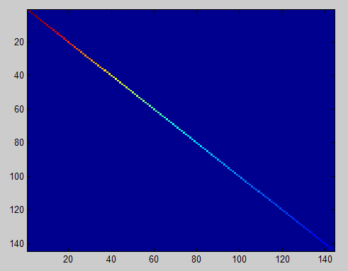
Step 1b: Check covariance

To verify that your implementation of PCA is correct, you should check the covariance matrix for the rotated data x_rot. PCA guarantees that the covariance matrix for the rotated data is a diagonal matrix (a matrix with non-zero entries only along the main diagonal). Implement code to compute the covariance matrix and verify this property. One way to do this is to compute the covariance matrix, and visualise it using the MATLAB command imagesc.

Step 2: Find number of components to retain

Next, choose k, the number of principal components to retain. Pick k to be as small as possible, but so that at least 99% of the variance is retained.

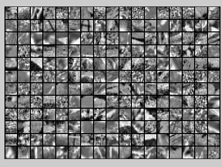
Step 3: PCA with dimension reduction

Now that you have found k, compute , the reduced-dimension representation of the data. This gives you a representation of each image patch as a k dimensional vector instead of a 144 dimensional vector.

Raw images

PCA dimension-reduced images
(99% variance)

PCA dimension-reduced images
(90% variance)

Step 4: PCA with whitening and regularization

Step 4a: Implement PCA with whitening and regularization

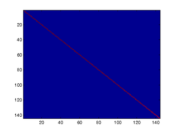
Step 4b: Check covariance

Similar to using PCA alone, PCA with whitening also results in processed data that has a diagonal covariance matrix. However, unlike PCA alone, whitening additionally ensures that the diagonal entries are equal to 1, i.e. that the covariance matrix is the identity matrix.That would be the case if you were doing whitening alone with no regularization. However, in this case you are whitening with regularization, to avoid numerical/etc. problems associated with small eigenvalues. As a result of this, some of the diagonal entries of the covariance of your x_PCAwhite will be smaller than 1.

Covariance for PCA whitening with regularization

Covariance for PCA whitening without regularization

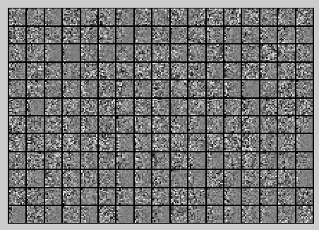
Step 5: ZCA whitening

Now implement ZCA whitening to produce the matrix x_ZCAWhite. Visualize x_ZCAWhite and compare it to the raw data

实验过程及结果

随机选取10000个patch，并显示其中204个patch，如下图所示：

然后对这些patch做均值为0化操作得到如下图：

对选取出的patch做PCA变换得到新的样本数据，其新样本数据的协方差矩阵如下图所示：

保留99%的方差后的PCA还原原始数据，如下所示：

PCA Whitening后的图像如下：

此时样本patch的协方差矩阵如下:

ZCA Whitening的结果如下：

Code

%%================================================================
%% Step 0a: Load data
%  Here we provide the code to load natural image data into x.
%  x will be a  *  matrix, where the kth column x(:, k) corresponds to
%  the raw image data from the kth 12x12 image patch sampled.
%  You do not need to change the code below.

x = sampleIMAGESRAW();
figure('name','Raw images');
randsel = randi(size(x,),,); % A random selection of samples for visualization
display_network(x(:,randsel));%为什么x有负数还可以显示？

%%================================================================
%% Step 0b: Zero-mean the data (by row)
%  You can make use of the mean and repmat/bsxfun functions.

% -------------------- YOUR CODE HERE --------------------
x = x-repmat(mean(x,),size(x,),);%求的是每一列的均值
%x = x-repmat(mean(x,),,size(x,));

%%================================================================
%% Step 1a: Implement PCA to obtain xRot
%  Implement PCA to obtain xRot, the matrix in which the data is expressed
%  with respect to the eigenbasis of sigma, which is the matrix U.

% -------------------- YOUR CODE HERE --------------------
xRot = zeros(size(x)); % You need to compute this
[n m] = size(x);
sigma = (1.0/m)*x*x';
[u s v] = svd(sigma);
xRot = u'*x;

%%================================================================
%% Step 1b: Check your implementation of PCA
%  The covariance matrix for the data expressed with respect to the basis U
%  should be a diagonal matrix with non-zero entries only along the main
%  diagonal. We will verify this here.
%  Write code to compute the covariance matrix, covar.
%  When visualised as an image, you should see a straight line across the
%  diagonal (non-zero entries) against a blue background (zero entries).

% -------------------- YOUR CODE HERE --------------------
covar = zeros(size(x, )); % You need to compute this
covar = (./m)*xRot*xRot';

% Visualise the covariance matrix. You should see a line across the
% diagonal against a blue background.
figure('name','Visualisation of covariance matrix');
imagesc(covar);

%%================================================================
%% Step : Find k, the number of components to retain
%  Write code to determine k, the number of components to retain in order
%  to retain at least % of the variance.

% -------------------- YOUR CODE HERE --------------------
k = ; % Set k accordingly
ss = diag(s);
% for k=:m
%    if sum(s(:k))./sum(ss) < 0.99
%        continue;
% end
%其中cumsum(ss)求出的是一个累积向量，也就是说ss向量值的累加值
%并且(cumsum(ss)/sum(ss))<=.99是一个向量，值为0或者1的向量，为1表示满足那个条件
k = length(ss((cumsum(ss)/sum(ss))<=0.99));

%%================================================================
%% Step : Implement PCA with dimension reduction
%  Now that you have found k, you can reduce the dimension of the data by
%  discarding the remaining dimensions. In this way, you can represent the
%  data in k dimensions instead of the original , which will save you
%  computational time when running learning algorithms on the reduced
%  representation.
%
%  Following the dimension reduction, invert the PCA transformation to produce
%  the matrix xHat, the dimension-reduced data with respect to the original basis.
%  Visualise the data and compare it to the raw data. You will observe that
%  there is little loss due to throwing away the principal components that
%  correspond to dimensions with low variation.

% -------------------- YOUR CODE HERE --------------------
xHat = zeros(size(x));  % You need to compute this
xHat = u*[u(:,:k)'*x;zeros(n-k,m)];

% Visualise the data, and compare it to the raw data
% You should observe that the raw and processed data are of comparable quality.
% For comparison, you may wish to generate a PCA reduced image which
% retains only % of the variance.

figure('name',['PCA processed images ',sprintf('(%d / %d dimensions)', k, size(x, )),'']);
display_network(xHat(:,randsel));
figure('name','Raw images');
display_network(x(:,randsel));

%%================================================================
%% Step 4a: Implement PCA with whitening and regularisation
%  Implement PCA with whitening and regularisation to produce the matrix
%  xPCAWhite. 

epsilon = 0.1;
xPCAWhite = zeros(size(x));

% -------------------- YOUR CODE HERE --------------------
xPCAWhite = diag(./sqrt(diag(s)+epsilon))*u'*x;
figure('name','PCA whitened images');
display_network(xPCAWhite(:,randsel));

%%================================================================
%% Step 4b: Check your implementation of PCA whitening
%  Check your implementation of PCA whitening with and without regularisation.
%  PCA whitening without regularisation results a covariance matrix
%  that is equal to the identity matrix. PCA whitening with regularisation
%  results in a covariance matrix with diagonal entries starting close to
%   and gradually becoming smaller. We will verify these properties here.
%  Write code to compute the covariance matrix, covar.
%
%  Without regularisation (set epsilon to  or close to ),
%  when visualised as an image, you should see a red line across the
%  diagonal (one entries) against a blue background (zero entries).
%  With regularisation, you should see a red line that slowly turns
%  blue across the diagonal, corresponding to the one entries slowly
%  becoming smaller.

% -------------------- YOUR CODE HERE --------------------
covar = (./m)*xPCAWhite*xPCAWhite';

% Visualise the covariance matrix. You should see a red line across the
% diagonal against a blue background.
figure('name','Visualisation of covariance matrix');
imagesc(covar);

%%================================================================
%% Step : Implement ZCA whitening
%  Now implement ZCA whitening to produce the matrix xZCAWhite.
%  Visualise the data and compare it to the raw data. You should observe
%  that whitening results in, among other things, enhanced edges.

xZCAWhite = zeros(size(x));

% -------------------- YOUR CODE HERE --------------------
xZCAWhite = u*xPCAWhite;

% Visualise the data, and compare it to the raw data.
% You should observe that the whitened images have enhanced edges.
figure('name','ZCA whitened images');
display_network(xZCAWhite(:,randsel));
figure('name','Raw images');
display_network(x(:,randsel));