Linear Regression with Scikit Learn

Before you read

This is a demo or practice about how to use Simple-Linear-Regression in scikit-learn with python. Following is the package version that I use below:

The Python version: 3.6.2

The Numpy version: 1.8.0rc1

The Scikit-Learn version: 0.19.0

The Matplotlib version: 2.0.2

Training Data

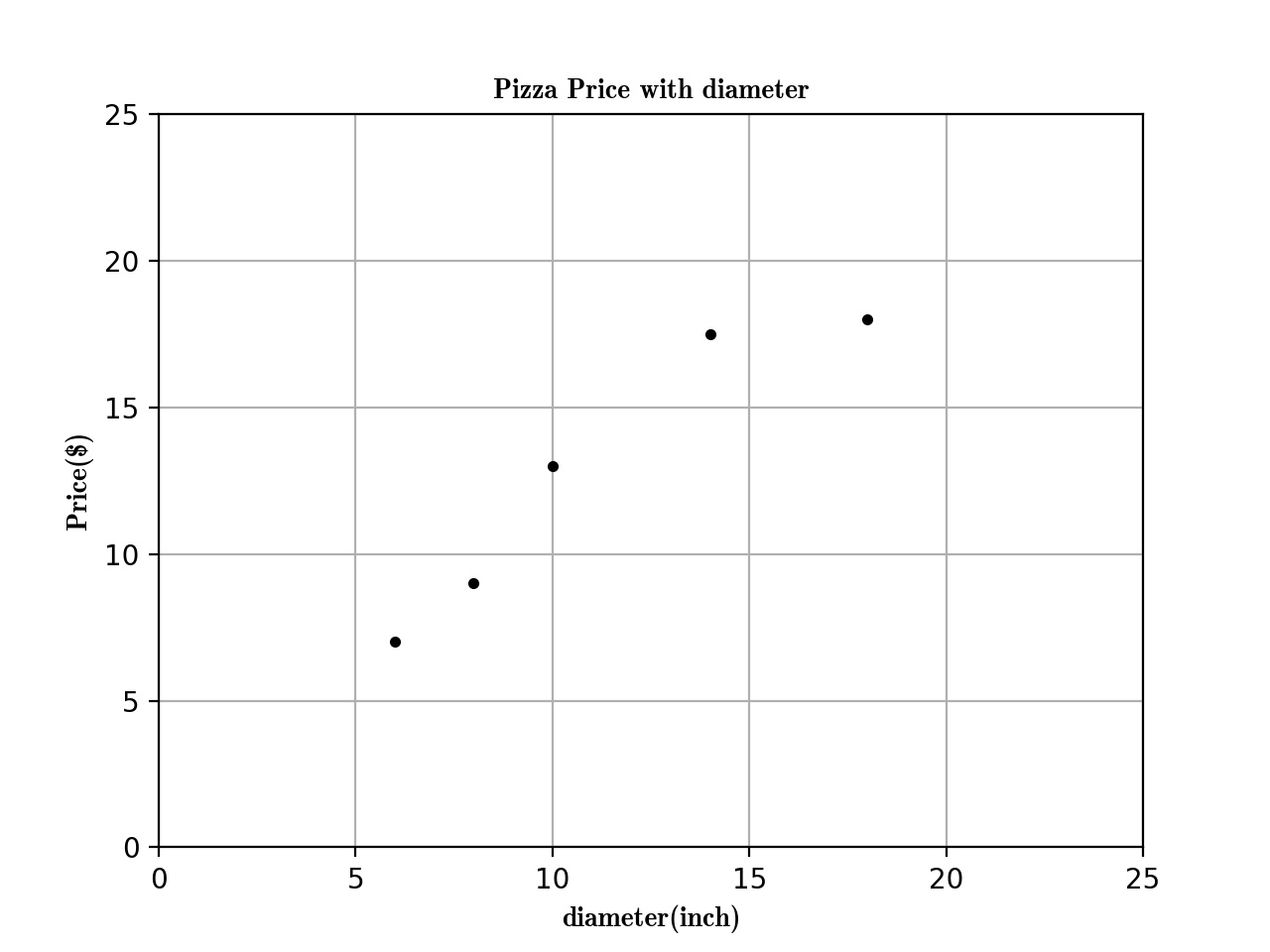
Here is the training data about the Relationship between Pizza and Diameter below:

training data	Diameter(inch)	Price($)
1	6	7
2	8	9
3	10	13
4	14	17.5
5	18	18

Now, we can plot the figure about the diameter and price first:

import matplotlib as plt

def run_plt():

    plt.figure()

    plt.title('Pizza Price with diameter.')

    plt.xlabel('diameter(inch)')

    plt.ylabel('price($)')

    plt.axis([0, 25, 0, 25])

    plt.grid(True)

    return plt

X = [[6], [8], [10], [14], [18]]

y = [[7], [9], [13], [17.5], [18]]

plt = run_plt()

plt.plot(X, y, 'k.')

plt.show()

Now we get the figure here.

Next, we use linear regression to fit this model.

from scikit.linear_model import LinearRegression

model = LinearRegression()

# X and y is the data in previous code.

model.fit(X, y)

# To predict the 12inch pizza price.

price = model.predict([12][0])

print('The 12 Pizza price: % .2f' % price)

# The 12 Pizza price: 13.68

The Simple Linear Regression define:

Simple linear regression assumes that a linear relationship exists between the response variable and explanatory variable; it models this relationship with a linear surface called a hyperplane. A hyperplane is a subspace that has one dimension less than the ambient space that contains it. In simple linear regression, there is one dimension for the response variable and another dimension for the explanatory variable, making a total of two dimensions. The regression hyperplane therefore, has one dimension; a hyperplane with one dimension is a line.

The Simple Linear Regression model that scikit-learn use is below:

$y = \alpha + \beta * x$

$y$ is the predicted value of the response variable. $x$ is the explanatory variable. $alpha$ and $beta$ are learned by the learning algorithm.

If we have a data $X_{2}$ like that,

$X_{2}$ = [[0], [10], [14], [25]]

We want to use Linear Regression to Predict the Prize Price and Print the Figure. There are two steps:

Use $x$, $y$ previous to fit the model.
Predict the Prize price.

model = LinearRegression()

# X, y is the prevoius data

model.fit(X,y)

X2 = [[0], [10], [14], [25]]

y2 = model.predict(X2)

plt.plot(X2, y2, 'g-')

The figure is following:

Summarize

The function previous that I used is called ordinary least squares. The process is :

Define the cost function and fit the training data.
Get the predict data.

Evaluating the fitness of a model with a cost function

There are serveral line created by different parmeters, and we got a question is that which one is the best-fitting regression line ?

plt = run_plt()

plt.plot(X, y, 'k.')

y3 = [14.25, 14.25, 14.25, 14.25]

y4 = y2 * 0.5 + 5

model.fit(X[1:-1], y[1:-1])

y5 = model.predict(X2)

plt.plot(X2, y2, 'g-.')

plt.plot(X2, y3, 'r-.')

plt.plot(X2, y4, 'y-.')

plt.plot(X2, y5, 'o-')

plt.show()

The Define of cost function

A cost function, also called a loss function, is used to de ne and measure the

error of a model. The differences between the prices predicted by the model andthe observed prices of the pizzas in the training set are called residuals or training errors. Later, we will evaluate a model on a separate set of test data; the differences between the predicted and observed values in the test data are called prediction errors or test errors.

The figure is like that:

The original data is black point, as we can see, the green line is the best-fitting regression line. But how computer know!!!!

So we should use some mathematic method to tell the computer which one is best-fitting.

model.fit(X, y)

yr = model.predict(X)

for idx, x in enumerate(X)

    plt.plot([x, x], [y[idx], yr[idx]], 'r-')

Next we plot the residuals figure.

We can use residual sum of squares to measure the fitness.

$SS_{res} = \sum _{i =1}^n(y_{i} - f(x_{i}))^{2}$

Use Numpy package to calculate the $SS_{res}$ value is 1.75

import numpy as np

SSres = np.mean((model.predict(X) - y)** 2)

Solving ordinary least squares for simple linear regression

Recall that simple linear regression is that:

$y = \alpha + \beta * x$

Our goal is to get the value of $alpha$ and $beta$. We will solve $beta$ first, we should calculate the variance of $x$ and covariance of $x$ and $y$.

Variance is a measure of how far a set of values is spread out. If all of the numbers in the set are equal, the variance of the set is zero.

$var(x) = \frac{\sum_{i=1}^n(x_{i} - \overline{x})^{2}}{n-1}$

$\overline{x}$ is the mean of x .

var = np.var(X, ddof =1)

# var = 23.2

Convariance is a measure of how much two variales change to together. If the value of variables increase together. their convariace is positive. If one variable tends to increase while the other decreases, their convariace is negative. If their is no linear relationship between the two variables, their convariance will be equals to zero.

$cov(x,y) = \frac{\sum_{i=1}^n(x_{i}-\overline{x})(y_{i}-\overline{y})}{n-1}$

import numpy as np

cov = np.cov([6, 8, 10, 14, 18], [7, 9, 13, 17.5, 18])[0][1]

Their is a formula solve $\beta$

$\beta = \frac{cov(x,y)}{var(x)}$

$\beta = \frac{22.65}{23.2} = 0.9762$

We can solve $\alpha$ as the following formula:

$\alpha = \overline{y} - \beta * \overline{x}$

$\alpha = 12.9 - 0.9762 * 11.2 =1.9655$

Summarize

The Regression formula is like following:

$y = 1.9655 + 0.9762 * x$