PELT(Per-Entity Load Tracking)

引言

对于Linux内核而言，做一款好的进程调度器是一项非常具有挑战性的任务，主要原因是在进行CPU资源分配的时候必须满足如下的需求：

1、它必须是公平的

2、快速响应

3、系统的throughput要高

4、功耗要小

其实你仔细分析上面的需求，这些目标其实是相互冲突的，但是用户在提需求的时候就是这么任性，他们期望所有的需求都满足，而且不管系统中的负荷情况如何。因此，纵观Linux内核调度器这些年的发展，各种调度器算法在内核中来来去去，这也就不足为奇了。当然，2007年，2.6.23版本引入“完全公平调度器”（CFS）之后，调度器相对变得稳定一些。最近一个最重大的变化是在3.8版中合并的Per-entity load tracking。

完美的调度算法需要一个能够预知未来的水晶球：只有当内核准确地推测出每个进程对系统的需求，她才能最佳地完成调度任务。不幸的是，硬件制造商推出各种性能强劲的处理器，但从来也不考虑预测进程负载的需求。在没有硬件支持的情况下，调度器只能祭出通用的预测大法：用“过去”预测“未来”，也就是说调度器是基于过去的调度信息来预测未来该进程对CPU的需求。而在这些调度信息中，每一个进程过去的“性能”信息是核心要考虑的因素。但有趣的是，虽然内核密切跟踪每个进程实际运行的时间，但它并不清楚每个进程对系统负载的贡献程度。

而Per-entity load tracking系统解决了这些问题。

PELT（Per-Entity Load Tracking）

是一套进程调度中，用于计算进程对系统产生多少负载的模型。

Scheduling Entity（调度实体）：其实就是一个进程，或者一组进程。

Load Tracking（负载跟踪）：统计调度实体对系统负载的总贡献。

其主要思想为：

将时间切分为以1ms为单位的period，为了便于计算，将1ms设置为1024us。

在一个单位period中，一个scheduling entity对系统的负载贡献，可以根据该entity处于runnable状态的时间进行计算。如果在该period中，runnable的时间为x，那么对系统负载的贡献=x/1024。

以上这个系统负载值也可能会超过1024us，这是因为我们会累积过去period中的负载。但是对于过去的负载，在计算时，需要乘上一个衰减因子（decay factor）。

如果我们用Li表示在周期Pi中该scheduling entity对系统负载的贡献，那么一个scheduling entity对系统负载的总贡献表示为：

L = L₀ + L₁*y + L₂*y² + L₃*y³ + ...

* [<-  1024us  ->|<-  1024us  ->|<-  1024us  ->| ...

*         P0                    P1                    P2           ...

*         L₀                     L₁                    L_{2              ...}

*        (now)          (~1ms ago)     (~2ms ago)

其中y就是衰减因子，从上面公式：

1. scheduling entity对于系统的负载贡献是一个幂级数之和。

2. 最近的负载的权重最大。

3. 过去的负载也会累计，但是会通过逐渐衰减的方式，影响负载计算。

使用这样序列的好处是计算简单，我们不需要使用数组来记录过去的负荷贡献，只要把上次的总负荷的贡献值乘以y再加上新的L0负荷值就OK了。

那么衰减因子y是多少呢？在3.8内核中，y^32=0.5，即32ms。32个period之后，负载的影响力为真实的一半。period计数超过32*63-1之后，就会清零load，也就是只会统计前64*63-1个perod的load。

那么最大的负载是多少呢？1024(1+y+y² + y³ + ... ) = 1024*(y/1-y) = 47742

runnable的scheduling entity的负载计算：

那么有了计算runnable scheduling entity负载贡献的方法，这个负荷值就可以向上传递，通过累加control group中的每一个scheduling entity负载可以得到该control group对应的scheduling entity的负载值。这样的算法不断的向上推进，可以得到整个系统的负载。

未处于runnable的scheduling entity的负载计算：

内核可以选择记录所有进入阻塞状态的进程，像往常一样衰减它们的负载贡献，并将其增加到总负载中。但这么做是非常耗费资源的。所以，3.8版本的调度器在每个cfs_rq（每个control group都有自己的cfs rq）数据结构中，维护一个“blocked load”的成员，这个成员记录了所有阻塞状态进程对系统负荷的贡献。

当一个进程阻塞了，它的负载会从总的运行负载值（runnable load）中减去并添加到总的阻塞负载值（blocked load）中。该负载可以以相同的方式衰减（即每个周期乘以y）。

当阻塞的进程再次转换成运行态时，其负载值（适当进行衰减）则转移到运行负荷上来。

因此，跟踪blocked load只是需要在进程状态转换过程中有一点计算量，调度器并不需要由于跟踪阻塞负载而遍历一个进入阻塞状态进程的链表。

对节流进程（throttled processes）的负载计算：

所谓节流进程是指那些在“CFS带宽控制器”（ CFS bandwidth controller）下控制运行的进程。当这些进程用完了本周期内的CPU时间，即使它们仍然在运行状态，即使CPU空闲，调度器并不会把CPU资源分配给它们。因此节流进程不会对系统造成负荷。正因为如此，当进程处于被节流状态的时候，它们对系统负荷的贡献值不应该按照runnable进程计算。在等待下一个周期到来之前，throttled processes不能获取cpu资源，因此它们的负荷贡献值会衰减。

PELT的好处：

1. 在没有增加调度器开销的情况下，调度器现在对每个进程和“调度进程组”对系统负载的贡献有了更清晰的认识。有了更精细的统计数据（指per entity负载值）。

2. 我们可以通过跟踪的per entity负载值做一些有用的事情。最明显的使用场景可能是用于负载均衡：即把runnable进程平均分配到系统的CPU上，使每个CPU承载大致相同的负载。如果内核知道每个进程对系统负载有多大贡献，它可以很容易地计算迁移到另一个CPU的效果。这样进程迁移的结果应该更准确，从而使得负载平衡不易出错。

3. small-task packing patch的目标是将“小”进程收集到系统中的部分CPU上，从而允许系统中的其他处理器进入低功耗模式。在这种情况下，显然我们需要一种方法来计算得出哪些进程是“小”的进程。利用per-entity load tracking，内核可以轻松的进行识别。

内核中的其他子系统也可以使用per entity负载值做一些“文章”。CPU频率调节器（CPU frequency governor）和功率调节器（CPU power governor）可以利用per entity负载值来猜测在不久的将来，系统需要提供多少的CPU计算能力。既然有了per-entity load tracking这样的基础设施，我们期待看到开发人员可以使用per-entity负载信息来优化系统的行为。虽然per-entity load tracking仍然不是一个能够预测未来的水晶球，但至少我们对当前的系统中的进程对CPU资源的需求有了更好的理解。

代码基于android-4.9-q，github：https://github.com/aosp-mirror/kernel_common/branches

路径：

kernel\sched\fair.c

__update_load_avg函数，用于计算一个进程对load的贡献。

相关重要结构体：

struct sched_avg

 /*
  * The load_avg/util_avg accumulates an infinite geometric series
  * (see __update_load_avg() in kernel/sched/fair.c).
  *
  * [load_avg definition]
  *
  *   load_avg = runnable% * scale_load_down(load)
  *
  * where runnable% is the time ratio that a sched_entity is runnable.
  * For cfs_rq, it is the aggregated load_avg of all runnable and
  * blocked sched_entities.
  *
  * load_avg may also take frequency scaling into account:
  *
  *   load_avg = runnable% * scale_load_down(load) * freq%
  *
  * where freq% is the CPU frequency normalized to the highest frequency.
  *
  * [util_avg definition]
  *
  *   util_avg = running% * SCHED_CAPACITY_SCALE
  *
  * where running% is the time ratio that a sched_entity is running on
  * a CPU. For cfs_rq, it is the aggregated util_avg of all runnable
  * and blocked sched_entities.
  *
  * util_avg may also factor frequency scaling and CPU capacity scaling:
  *
  *   util_avg = running% * SCHED_CAPACITY_SCALE * freq% * capacity%
  *
  * where freq% is the same as above, and capacity% is the CPU capacity
  * normalized to the greatest capacity (due to uarch differences, etc).
  *
  * N.B., the above ratios (runnable%, running%, freq%, and capacity%)
  * themselves are in the range of [0, 1]. To do fixed point arithmetics,
  * we therefore scale them to as large a range as necessary. This is for
  * example reflected by util_avg's SCHED_CAPACITY_SCALE.
  *
  * [Overflow issue]
  *
  * The 64-bit load_sum can have 4353082796 (=2^64/47742/88761) entities
  * with the highest load (=88761), always runnable on a single cfs_rq,
  * and should not overflow as the number already hits PID_MAX_LIMIT.
  *
  * For all other cases (including 32-bit kernels), struct load_weight's
  * weight will overflow first before we do, because:
  *
  *    Max(load_avg) <= Max(load.weight)
  *
  * Then it is the load_weight's responsibility to consider overflow
  * issues.
  */
 struct sched_avg {
     u64 last_update_time, load_sum;
     u32 util_sum, period_contrib;
     unsigned long load_avg, util_avg;
 };

 /*
  * We can represent the historical contribution to runnable average as the
  * coefficients of a geometric series.  To do this we sub-divide our runnable
  * history into segments of approximately 1ms (1024us); label the segment that
  * occurred N-ms ago p_N, with p_0 corresponding to the current period, e.g.
  *
  * [<- 1024us ->|<- 1024us ->|<- 1024us ->| ...
  *      p0            p1           p2
  *     (now)       (~1ms ago)  (~2ms ago)
  *
  * Let u_i denote the fraction of p_i that the entity was runnable.
  *
  * We then designate the fractions u_i as our co-efficients, yielding the
  * following representation of historical load:
  *   u_0 + u_1*y + u_2*y^2 + u_3*y^3 + ...
  *
  * We choose y based on the with of a reasonably scheduling period, fixing:
  *   y^32 = 0.5
  *
  * This means that the contribution to load ~32ms ago (u_32) will be weighted
  * approximately half as much as the contribution to load within the last ms
  * (u_0).
  *
  * When a period "rolls over" and we have new u_0`, multiplying the previous
  * sum again by y is sufficient to update:
  *   load_avg = u_0` + y*(u_0 + u_1*y + u_2*y^2 + ... )
  *            = u_0 + u_1*y + u_2*y^2 + ... [re-labeling u_i --> u_{i+1}]
  */

     |                  n*Period             |    P_n+      |      P_n+   |
 |---|---------------------------------------|----|----------|--------------|
 T0  T1                                      T2   T3         T4
 |                                                |
 current_time                                     last_time

 static __always_inline int
 __update_load_avg(u64 now, int cpu, struct sched_avg *sa,
           unsigned long weight, int running, struct cfs_rq *cfs_rq)
 {
     u64 delta, scaled_delta, periods;
     u32 contrib;
     unsigned int delta_w, scaled_delta_w, decayed = ;
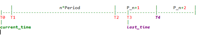
     unsigned long scale_freq, scale_cpu;

     delta = now - sa->last_update_time;//计算delta时间= current_time - last_time
     /*
      * This should only happen when time goes backwards, which it
      * unfortunately does during sched clock init when we swap over to TSC.
      */
     if ((s64)delta < ) {
         sa->last_update_time = now;
         return ;
     }

     /*
      * Use 1024ns as the unit of measurement since it's a reasonable
      * approximation of 1us and fast to compute.
      */
     delta >>= ;    //将ns转化为us，确认delta >= 1024ns（单位时间period），才可以更新
     if (!delta)
         return ;
     sa->last_update_time = now; //为下次计算delta做准备

     scale_freq = arch_scale_freq_capacity(NULL, cpu);  //获取不同freq影响因子,当前freq 相对 本cpu最大freq 的比值：scale_freq = (cpu_curr_freq / cpu_max_freq) * 1024
     scale_cpu = arch_scale_cpu_capacity(NULL, cpu);       //获取不同CPU影响因子,表示 (当前cpu最大运算能力 相对 所有cpu中最大的运算能力 的比值) * (cpufreq_policy的最大频率 相对 本cpu最大频率 的比值)，：scale_cpu = cpu_scale * max_freq_scale / 1024。cpu_scale表示 当前cpu最大运算能力 相对 所有cpu中最大的运算能力 的比值：cpu_scale = ((cpu_max_freq * efficiency) / max_cpu_perf) * 1024
     trace_sched_contrib_scale_f(cpu, scale_freq, scale_cpu);

     /* delta_w is the amount already accumulated against our next period */
     delta_w = sa->period_contrib;
     if (delta + delta_w >= ) {    //如果出现时间长度超过period（1ms），那么在计算当前load的时候，上一个period中的load需要乘上衰减系数
         decayed = ;

         /* how much left for next period will start over, we don't know yet */
         sa->period_contrib = ;

         /*
          * Now that we know we're crossing a period boundary, figure
          * out how much from delta we need to complete the current
          * period and accrue it.
          */
         delta_w =  - delta_w;    //补齐上一个period的部分: T2-T3
         scaled_delta_w = cap_scale(delta_w, scale_freq); // (delta_w * scale_freq) >> 10， 计算该部分的load * freq
         if (weight) {
             sa->load_sum += weight * scaled_delta_w;    // weight * load * freq , 将结果累计到sa->load_sum中
             if (cfs_rq) {
                 cfs_rq->runnable_load_sum +=
                         weight * scaled_delta_w;        //同时也累计到cfs_rq->runnable_load_sum中
             }
         }
         if (running)
             sa->util_sum += scaled_delta_w * scale_cpu; //如果进程当前状态是running，那么也累计到sa->util_sum中

         delta -= delta_w;        //去掉补齐部分,剩下需要计算的load: current time-T2 

         /* Figure out how many additional periods this update spans */
         periods = delta / ;        //计算n的值
         delta %= ;                //计算T0-T1

         sa->load_sum = decay_load(sa->load_sum, periods + );//计算T2以前load到当前perdiod时影响：以前的load * 衰减y^（period+1）, 将结果累计到sa->load_sum中。当period+1> 64*63时，load为0,
         if (cfs_rq) {
             cfs_rq->runnable_load_sum =
                 decay_load(cfs_rq->runnable_load_sum, periods + ); //统计cfs_rq->runnable_load_sum中
         }
         sa->util_sum = decay_load((u64)(sa->util_sum), periods + );//如果进程当前状态是running，那么也累计到sa->util_sum中

         /* Efficiently calculate \sum (1..n_period) 1024*y^i */
         contrib = __compute_runnable_contrib(periods);    //计算n个period的load
         contrib = cap_scale(contrib, scale_freq);    //(delta_w * scale_freq) >> 10， 计算该部分的load * freq
         if (weight) {
             sa->load_sum += weight * contrib;        //weight * load * freq , 将结果累计到sa->load_sum中
             if (cfs_rq)
                 cfs_rq->runnable_load_sum += weight * contrib; //同时也累计到cfs_rq->runnable_load_sum中
         }
         if (running)
             sa->util_sum += contrib * scale_cpu;    //如果进程当前状态是running，那么也累计到sa->util_sum中
     }

     /* Remainder of delta accrued against u_0` */
     scaled_delta = cap_scale(delta, scale_freq);    //计算T0-T1的load，并考虑cpu freq影响
     if (weight) {
         sa->load_sum += weight * scaled_delta;    //考虑weight的影响，结果统计到sa->load_sum中
         if (cfs_rq)
             cfs_rq->runnable_load_sum += weight * scaled_delta;    //将结果统计到cfs->runnable_load_sum中，并考虑weight影响
     }
     if (running)
         sa->util_sum += scaled_delta * scale_cpu;    //如果是runnable进程，同时将结果统计到sa->util_sum中

     sa->period_contrib += delta;    //将未满1个period的时间，暂存起来。这里与上面71行代码对应

     if (decayed) {    //至少计算时，包好一个完整period
         sa->load_avg = div_u64(sa->load_sum, LOAD_AVG_MAX);    //计算load_avg，用当前load/load_max，计算得出一个百分比结果，表示当前的平均load
         if (cfs_rq) {
             cfs_rq->runnable_load_avg =
                 div_u64(cfs_rq->runnable_load_sum, LOAD_AVG_MAX);    //同样方法计算cfs_rq->runnable_load_sum的平均load
         }
         sa->util_avg = sa->util_sum / LOAD_AVG_MAX;    //同样方法计算sa->util_sum的平均load
     }

     return decayed;
 }

看到以上代码中，有3个统计数据，分别为：

sa->load_sum：统计所有类型和状态下的load（考虑了freq scale，weight）

cfs_rq->runnable_load_sum：仅统计属于cfs_rq的load（考虑了freq scale，weight）

sa->util_sum：仅统计处于running状态的load（考虑了cpu scale）

最后分别除以LOAD_AVG_MAX，计算除对应的load_avg：

sa->load_avg = div_u64(sa->load_sum, LOAD_AVG_MAX);
cfs_rq->runnable_load_avg =div_u64(cfs_rq->runnable_load_sum, LOAD_AVG_MAX);
sa->util_avg = sa->util_sum / LOAD_AVG_MAX;

前面2个，考虑了weight的影响，实际目的是：加入了weight的归一化。即认为两个不同的task，其运行时间是一样的，由于优先级/weight的不同，其对于runqueue的load的贡献值也不同。

而cpu scale表示了因不同CPU架构而体现出不同的cpu capacity。这会为后续的task placement作为参考。

预定义了最大的period长度：32

最大的load值：47742

当一个100%的进程，运行345ms后，就可以达到load最大值

 /*
  * We choose a half-life close to 1 scheduling period.
  * Note: The tables runnable_avg_yN_inv and runnable_avg_yN_sum are
  * dependent on this value.
  */
 #define LOAD_AVG_PERIOD 32
 #define LOAD_AVG_MAX 47742 /* maximum possible load avg */
 #define LOAD_AVG_MAX_N 345 /* number of full periods to produce LOAD_AVG_MAX */

预配置的load数组，为了减少计算量：

 /* Precomputed fixed inverse multiplies for multiplication by y^n */
 static const u32 runnable_avg_yN_inv[] = {
     0xffffffff, 0xfa83b2da, 0xf5257d14, 0xefe4b99a, 0xeac0c6e6, 0xe5b906e6,
     0xe0ccdeeb, 0xdbfbb796, 0xd744fcc9, 0xd2a81d91, 0xce248c14, 0xc9b9bd85,
     0xc5672a10, 0xc12c4cc9, 0xbd08a39e, 0xb8fbaf46, 0xb504f333, 0xb123f581,
     0xad583ee9, 0xa9a15ab4, 0xa5fed6a9, 0xa2704302, 0x9ef5325f, 0x9b8d39b9,
     0x9837f050, 0x94f4efa8, 0x91c3d373, 0x8ea4398a, 0x8b95c1e3, 0x88980e80,
     0x85aac367, 0x82cd8698,
 };

 /*
  * Precomputed \Sum y^k { 1<=k<=n }.  These are floor(true_value) to prevent
  * over-estimates when re-combining.
  */
 static const u32 runnable_avg_yN_sum[] = {
         , , , , , , , , , , ,
      ,,,,,,,,,,,
     ,,,,,,,,,,,
 };

 /*
  * Precomputed \Sum y^k { 1<=k<=n, where n%32=0). Values are rolled down to
  * lower integers. See Documentation/scheduler/sched-avg.txt how these
  * were generated:
  */
 static const u32 __accumulated_sum_N32[] = {
         , , , , , ,
     , , , , , ,
 };

以下这个函数，是计算load（val）在经过（n）个period的衰减后，还剩多少影响。

 /*
  * Approximate:
  *   val * y^n,    where y^32 ~= 0.5 (~1 scheduling period)
  */
 static __always_inline u64 decay_load(u64 val, u64 n)
 {
     unsigned int local_n;

     if (!n)
         return val;
     else if (unlikely(n > LOAD_AVG_PERIOD * )) //[32] * 63
         return ;

     /* after bounds checking we can collapse to 32-bit */
     local_n = n;

     /*
      * As y^PERIOD = 1/2, we can combine
      *    y^n = 1/2^(n/PERIOD) * y^(n%PERIOD)
      * With a look-up table which covers y^n (n<PERIOD)
      *
      * To achieve constant time decay_load.
      */
     if (unlikely(local_n >= LOAD_AVG_PERIOD)) {
         val >>= local_n / LOAD_AVG_PERIOD;
         local_n %= LOAD_AVG_PERIOD;
     }

     val = mul_u64_u32_shr(val, runnable_avg_yN_inv[local_n], );
     return val;
 }

 /*
  * For updates fully spanning n periods, the contribution to runnable
  * average will be: \Sum 1024*y^n
  *
  * We can compute this reasonably efficiently by combining:
  *   y^PERIOD = 1/2 with precomputed \Sum 1024*y^n {for  n <PERIOD}
  */
 static u32 __compute_runnable_contrib(u64 n)
 {
     u32 contrib = ;

     if (likely(n <= LOAD_AVG_PERIOD))
         return runnable_avg_yN_sum[n];
     else if (unlikely(n >= LOAD_AVG_MAX_N))
         return LOAD_AVG_MAX;

     /* Since n < LOAD_AVG_MAX_N, n/LOAD_AVG_PERIOD < 11 */
     contrib = __accumulated_sum_N32[n/LOAD_AVG_PERIOD];
     n %= LOAD_AVG_PERIOD;
     contrib = decay_load(contrib, n);
     return contrib + runnable_avg_yN_sum[n];
 }

代码分析综述：

从代码解析来看，实际整个函数其实只是完成了在不同阶段时，load的计算和统计的一半方法，并得出平均load。

关键在于load计算出来后，运用在什么场景下，这块我还没有完善。当然，我们是知道用于负载均衡的。同时我们从3个统计数据，也可以看出一些端倪，有2个是考虑了freq_scale和weight，有1个是考虑了cpu_scale。可能会用于任务migration。

具体后续会另起blog。

参考：

http://www.wowotech.net/process_management/PELT.html

https://lwn.net/Articles/531853/

https://www.anandtech.com/show/8933/snapdragon-810-performance-preview/4