chapter3——逻辑回归手动+sklean版本

1 导入numpy包

import numpy as np

2 sigmoid函数

def sigmoid(x):
    return 1/(1+np.exp(-x))
demox = np.array([1,2,3])
print(sigmoid(demox))
#报错
#demox = [1,2,3]
# print(sigmoid(demox))

结果：

[0.73105858 0.88079708 0.95257413]

3 定义逻辑回归模型主体

### 定义逻辑回归模型主体
def logistic(x, y, w, b):
    # 训练样本量
    num_train = x.shape[0]
    # 逻辑回归模型输出
    y_hat = sigmoid(np.dot(x,w)+b)
    # 交叉熵损失
    cost = -1/(num_train)*(np.sum(y*np.log(y_hat)+(1-y)*np.log(1-y_hat)))
    # 权值梯度
    dW = np.dot(x.T,(y_hat-y))/num_train
    # 偏置梯度
    db = np.sum(y_hat- y)/num_train
    # 压缩损失数组维度
    cost = np.squeeze(cost)
    return y_hat, cost, dW, db

4 初始化函数

def init_parm(dims):
    w = np.zeros((dims,1))
    b = 0
    return w ,b 

5 定义逻辑回归模型训练过程

### 定义逻辑回归模型训练过程
def logistic_train(X, y, learning_rate, epochs):
    # 初始化模型参数
    W, b = init_parm(X.shape[1])
    cost_list = []
    for i in range(epochs):
        # 计算当前次的模型计算结果、损失和参数梯度
        a, cost, dW, db = logistic(X, y, W, b)
        # 参数更新
        W = W -learning_rate * dW
        b = b -learning_rate * db
        if i % 100 == 0:
            cost_list.append(cost)
        if i % 100 == 0:
            print('epoch %d cost %f' % (i, cost))
    params = {
        'W': W,
        'b': b
    }
    grads = {
        'dW': dW,
        'db': db
    }
    return cost_list, params, grads

6 定义预测函数

def predict(X,params):
    y_pred = sigmoid(np.dot(X,params['W'])+params['b'])
    y_preds = [1 if y_pred[i]>0.5 else 0 for i in range(len(y_pred))]
    return y_preds

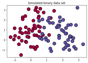
7 生成数据

# 导入matplotlib绘图库
import matplotlib.pyplot as plt
# 导入生成分类数据函数
from sklearn.datasets import make_classification
# 生成100*2的模拟二分类数据集
x ,label  = make_classification(
    n_samples=100,# 样本个数
    n_classes=2,# 样本类别
    n_features=2,#特征个数
    n_redundant=0,#冗余特征个数（有效特征的随机组合）
    n_informative=2,#有效特征，有价值特征
    n_repeated=0, # 重复特征个数（有效特征和冗余特征的随机组合）
    n_clusters_per_class=2 ,# 簇的个数
    random_state=1,
)
print("x.shape =",x.shape)
print("label.shape = ",label.shape)
print("np.unique(label) =",np.unique(label))
print(set(label))
# 设置随机数种子
rng = np.random.RandomState(2)
# 对生成的特征数据添加一组均匀分布噪声https://blog.csdn.net/vicdd/article/details/52667709
x += 2*rng.uniform(size=x.shape)
# 标签类别数
unique_label  = set(label)
# 根据标签类别数设置颜色
print(np.linspace(0,1,len(unique_label)))
colors = plt.cm.Spectral(np.linspace(0,1,len(unique_label)))
print(colors)
# 绘制模拟数据的散点图
for k,col in zip(unique_label , colors):
    x_k=x[label==k]
    plt.plot(x_k[:,0],x_k[:,1],'o',markerfacecolor=col,markeredgecolor="k",
             markersize=14)
plt.title('Simulated binary data set')
plt.show();

结果：

x.shape = (100, 2)
label.shape =  (100,)
np.unique(label) = [0 1]
{0, 1}
[0. 1.]
[[0.61960784 0.00392157 0.25882353 1.        ]
 [0.36862745 0.30980392 0.63529412 1.        ]]

　　　　

复习

# 复习
mylabel = label.reshape((-1,1))
data = np.concatenate((x,mylabel),axis=1)
print(data.shape)

结果：

(100, 3)

8 划分数据集

offset = int(x.shape[0]*0.7)
x_train, y_train = x[:offset],label[:offset].reshape((-1,1))
x_test, y_test = x[offset:],label[offset:].reshape((-1,1))
print(x_train.shape)
print(y_train.shape)
print(x_test.shape)
print(y_test.shape)

结果：

(70, 2)
(70, 1)
(30, 2)
(30, 1)

9 训练

cost_list, params, grads = logistic_train(x_train, y_train, 0.01, 1000)
print(params['b'])

结果：

epoch 0 cost 0.693147
epoch 100 cost 0.568743
epoch 200 cost 0.496925
epoch 300 cost 0.449932
epoch 400 cost 0.416618
epoch 500 cost 0.391660
epoch 600 cost 0.372186
epoch 700 cost 0.356509
epoch 800 cost 0.343574
epoch 900 cost 0.332689
-0.6646648941379839

10 准确率计算

from sklearn.metrics import accuracy_score,classification_report
y_pred = predict(x_test,params)
print("y_pred = ",y_pred)
print(y_pred)
print(y_test.shape)
print(accuracy_score(y_pred,y_test)) #不需要都是1维的，貌似会自动squeeze()
print(classification_report(y_test,y_pred))

结果：

y_pred =  [0, 0, 1, 1, 1, 1, 0, 0, 0, 1, 1, 1, 0, 1, 1, 1, 1, 1, 1, 0, 0, 1, 1, 0, 1, 1, 0, 0, 1, 0]
[0, 0, 1, 1, 1, 1, 0, 0, 0, 1, 1, 1, 0, 1, 1, 1, 1, 1, 1, 0, 0, 1, 1, 0, 1, 1, 0, 0, 1, 0]
(30, 1)
0.9333333333333333
              precision    recall  f1-score   support

           0       0.92      0.92      0.92        12
           1       0.94      0.94      0.94        18

    accuracy                           0.93        30
   macro avg       0.93      0.93      0.93        30
weighted avg       0.93      0.93      0.93        30

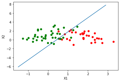
11 绘制逻辑回归决策边界

### 绘制逻辑回归决策边界
def plot_logistic(X_train, y_train, params):
    # 训练样本量
    n = X_train.shape[0]
    xcord1,ycord1,xcord2,ycord2 = [],[],[],[]
    # 获取两类坐标点并存入列表
    for i in range(n):
        if y_train[i] == 1:
            xcord1.append(X_train[i][0])
            ycord1.append(X_train[i][1])
        else:
            xcord2.append(X_train[i][0])
            ycord2.append(X_train[i][1])
    fig = plt.figure()
    ax = fig.add_subplot(111)
    ax.scatter(xcord1,ycord1,s = 30,c = 'red')
    ax.scatter(xcord2,ycord2,s = 30,c = 'green')
    # 取值范围
    x =np.arange(-1.5,3,0.1)
    # 决策边界公式
    y = (-params['b'] - params['W'][0] * x) / params['W'][1]
    # 绘图
    ax.plot(x, y)
    plt.xlabel('X1')
    plt.ylabel('X2')
    plt.show()
plot_logistic(x_train, y_train, params)

结果：

　　　　

11 sklearn实现

from sklearn.linear_model import LogisticRegression
clf = LogisticRegression(random_state=0).fit(x_train,y_train)
y_pred = clf.predict(x_test)
print(y_pred)
accuracy_score(y_test,y_pred)

结果：

[0 0 1 1 1 1 0 0 0 1 1 1 0 1 1 0 0 1 1 0 0 1 1 0 1 1 0 0 1 0]
0.9333333333333333