Best packages for data manipulation in R

dplyr and data.table are amazing packages that make data manipulation in R fun. Both packages have their strengths. While dplyr is more elegant and resembles natural language, data.table is succinct and we can do a lot withdata.table in just a single line. Further, data.table is, in some cases, faster (see benchmark here) and it may be a go-to package when performance and memory are constraints. You can read comparison of dplyr and data.tablefrom Stack Overflow and Quora.

You can get reference manual and vignettes for data.table here and for dplyrhere. You can read other tutorial about dplyr published at DataScience+

Background

I am a long time dplyr and data.table user for my data manipulation tasks. For someone who knows one of these packages, I thought it could help to show codes that perform the same tasks in both packages to help them quickly study the other. If you know either package and have interest to study the other, this post is for you.

dplyr

dplyr has 5 verbs which make up the majority of the data manipulation tasks we perform. Select: used to select one or more columns; Filter: used to select some rows based on specific criteria; Arrange: used to sort data based on one or more columns in ascending or descending order; Mutate: used to add new columns to our data; Summarise: used to create chunks from our data.

data.table

data.table has a very succinct general format: DT[i, j, by], which is interpreted as: Take DT, subset rows using i, then calculate j grouped by by.

Data manipulation

First we will install some packages for our project.

library(dplyr)
library(data.table)
library(lubridate)
library(jsonlite)
library(tidyr)
library(ggplot2)
library(compare)

The data we will use here is from DATA.GOV. It is Medicare Hospital Spending by Claim and it can be downloaded from here. Let’s download the data in JSONformat using the fromJSON function from the jsonlite package. Since JSON is a very common data format used for asynchronous browser/server communication, it is good if you understand the lines of code below used to get the data. You can get an introductory tutorial on how to use the jsonlite package to work with JSON data here and here. However, if you want to focus only on the data.table and dplyr commands, you can safely just run the codes in the two cells below and ignore the details.

spending=fromJSON("https://data.medicare.gov/api/views/nrth-mfg3/rows.json?accessType=DOWNLOAD")
names(spending)
"meta" "data" 

meta=spending$meta
hospital_spending=data.frame(spending$data)
colnames(hospital_spending)=make.names(meta$view$columns$name)
hospital_spending=select(hospital_spending,-c(sid:meta))

glimpse(hospital_spending)
Observations: 70598
Variables:
$ Hospital.Name                       (fctr) SOUTHEAST ALABAMA MEDICAL CENT...
$ Provider.Number.                    (fctr) 010001, 010001, 010001, 010001...
$ State                               (fctr) AL, AL, AL, AL, AL, AL, AL, AL...
$ Period                              (fctr) 1 to 3 days Prior to Index Hos...
$ Claim.Type                          (fctr) Home Health Agency, Hospice, I...
$ Avg.Spending.Per.Episode..Hospital. (fctr) 12, 1, 6, 160, 1, 6, 462, 0, 0...
$ Avg.Spending.Per.Episode..State.    (fctr) 14, 1, 6, 85, 2, 9, 492, 0, 0,...
$ Avg.Spending.Per.Episode..Nation.   (fctr) 13, 1, 5, 117, 2, 9, 532, 0, 0...
$ Percent.of.Spending..Hospital.      (fctr) 0.06, 0.01, 0.03, 0.84, 0.01, ...
$ Percent.of.Spending..State.         (fctr) 0.07, 0.01, 0.03, 0.46, 0.01, ...
$ Percent.of.Spending..Nation.        (fctr) 0.07, 0.00, 0.03, 0.58, 0.01, ...
$ Measure.Start.Date                  (fctr) 2014-01-01T00:00:00, 2014-01-0...
$ Measure.End.Date                    (fctr) 2014-12-31T00:00:00, 2014-12-3...

As shown above, all columns are imported as factors and let’s change the columns that contain numeric values to numeric.

cols = 6:11; # These are the columns to be changed to numeric.
hospital_spending[,cols] <- lapply(hospital_spending[,cols], as.numeric)

The last two columns are measure start date and measure end date. So, let’s use the lubridate package to correct the classes of these columns.

cols = 12:13; # These are the columns to be changed to dates.
hospital_spending[,cols] <- lapply(hospital_spending[,cols], ymd_hms)

Now, let’s check if the columns have the classes we want.

sapply(hospital_spending, class)
$Hospital.Name
    "factor"
$Provider.Number.
    "factor"
$State
    "factor"
$Period
    "factor"
$Claim.Type
    "factor"
$Avg.Spending.Per.Episode..Hospital.
    "numeric"
$Avg.Spending.Per.Episode..State.
    "numeric"
$Avg.Spending.Per.Episode..Nation.
    "numeric"
$Percent.of.Spending..Hospital.
    "numeric"
$Percent.of.Spending..State.
    "numeric"
$Percent.of.Spending..Nation.
    "numeric"
$Measure.Start.Date
        "POSIXct" "POSIXt"
$Measure.End.Date
        "POSIXct" "POSIXt"

Create data table

We can create a data.table using the data.table() function.

hospital_spending_DT = data.table(hospital_spending)
class(hospital_spending_DT)
"data.table" "data.frame" 

Select certain columns of data

To select columns, we use the verb select in dplyr. In data.table, on the other hand, we can specify the column names.

Selecting one variable

Let’s selet the “Hospital Name” variable

from_dplyr = select(hospital_spending, Hospital.Name)
from_data_table = hospital_spending_DT[,.(Hospital.Name)]

Now, let’s compare if the results from dplyr and data.table are the same.

compare(from_dplyr,from_data_table, allowAll=TRUE)
TRUE
dropped attributes

Removing one variable

from_dplyr = select(hospital_spending, -Hospital.Name)
from_data_table = hospital_spending_DT[,!c("Hospital.Name"),with=FALSE]
compare(from_dplyr,from_data_table, allowAll=TRUE)
TRUE
dropped attributes

we can also use := function which modifies the input data.table by reference.
We will use the copy() function, which deep copies the input object and therefore any subsequent update by reference operations performed on the copied object will not affect the original object.

DT=copy(hospital_spending_DT)
DT=DT[,Hospital.Name:=NULL]
"Hospital.Name"%in%names(DT)FALSE 

We can also remove many variables at once similarly:

DT=copy(hospital_spending_DT)
DT=DT[,c("Hospital.Name","State","Measure.Start.Date","Measure.End.Date"):=NULL]
c("Hospital.Name","State","Measure.Start.Date","Measure.End.Date")%in%names(DT)
FALSE FALSE FALSE FALSE 

Selecting multiple variables

Let’s select the variables:
Hospital.Name,State,Measure.Start.Date,and Measure.End.Date.

from_dplyr = select(hospital_spending, Hospital.Name,State,Measure.Start.Date,Measure.End.Date)
from_data_table = hospital_spending_DT[,.(Hospital.Name,State,Measure.Start.Date,Measure.End.Date)]
compare(from_dplyr,from_data_table, allowAll=TRUE)
TRUE
dropped attributes

Dropping multiple variables

Now, let’s remove the variables Hospital.Name,State,Measure.Start.Date,and Measure.End.Date from the original data frame hospital_spending and the data.table hospital_spending_DT.

from_dplyr = select(hospital_spending, -c(Hospital.Name,State,Measure.Start.Date,Measure.End.Date))
from_data_table = hospital_spending_DT[,!c("Hospital.Name","State","Measure.Start.Date","Measure.End.Date"),with=FALSE]
compare(from_dplyr,from_data_table, allowAll=TRUE)
TRUE
dropped attributes

dplyr has functions contains(), starts_with() and, ends_with() which we can use with the verb select. In data.table, we can use regular expressions. Let’s select columns that contain the word Date to demonstrate by example.

from_dplyr = select(hospital_spending,contains("Date"))
from_data_table = subset(hospital_spending_DT,select=grep("Date",names(hospital_spending_DT)))
compare(from_dplyr,from_data_table, allowAll=TRUE)
TRUE
dropped attributes

names(from_dplyr)
"Measure.Start.Date" "Measure.End.Date" 

Rename columns

setnames(hospital_spending_DT,c("Hospital.Name", "Measure.Start.Date","Measure.End.Date"), c("Hospital","Start_Date","End_Date"))
names(hospital_spending_DT)
"Hospital" "Provider.Number." "State" "Period" "Claim.Type" "Avg.Spending.Per.Episode..Hospital." "Avg.Spending.Per.Episode..State." "Avg.Spending.Per.Episode..Nation." "Percent.of.Spending..Hospital." "Percent.of.Spending..State." "Percent.of.Spending..Nation." "Start_Date" "End_Date" 

hospital_spending = rename(hospital_spending,Hospital= Hospital.Name, Start_Date=Measure.Start.Date,End_Date=Measure.End.Date)
compare(hospital_spending,hospital_spending_DT, allowAll=TRUE)
TRUE
  dropped attributes

Filtering data to select certain rows

To filter data to select specific rows, we use the verb filter from dplyr with logical statements that could include regular expressions. In data.table, we need the logical statements only.

Filter based on one variable

from_dplyr = filter(hospital_spending,State=='CA') # selecting rows for California
from_data_table = hospital_spending_DT[State=='CA']
compare(from_dplyr,from_data_table, allowAll=TRUE)
TRUE
  dropped attributes

Filter based on multiple variables

from_dplyr = filter(hospital_spending,State=='CA' & Claim.Type!="Hospice")
from_data_table = hospital_spending_DT[State=='CA' & Claim.Type!="Hospice"]
compare(from_dplyr,from_data_table, allowAll=TRUE)
TRUE
  dropped attributes

from_dplyr = filter(hospital_spending,State %in% c('CA','MA',"TX"))
from_data_table = hospital_spending_DT[State %in% c('CA','MA',"TX")]
unique(from_dplyr$State)
CA MA TX 

compare(from_dplyr,from_data_table, allowAll=TRUE)
TRUE
dropped attributes

Order data

We use the verb arrange in dplyr to order the rows of data. We can order the rows by one or more variables. If we want descending, we have to use desc()as shown in the examples.The examples are self-explanatory on how to sort in ascending and descending order. Let’s sort using one variable.

Ascending

from_dplyr = arrange(hospital_spending, State)
from_data_table = setorder(hospital_spending_DT, State)
compare(from_dplyr,from_data_table, allowAll=TRUE)
TRUE
dropped attributes

Descending

from_dplyr = arrange(hospital_spending, desc(State))
from_data_table = setorder(hospital_spending_DT, -State)
compare(from_dplyr,from_data_table, allowAll=TRUE)
TRUE
dropped attributes

Sorting with multiple variables

Let’s sort with State in ascending order and End_Date in descending order.

from_dplyr = arrange(hospital_spending, State,desc(End_Date))
from_data_table = setorder(hospital_spending_DT, State,-End_Date)
compare(from_dplyr,from_data_table, allowAll=TRUE)
TRUE
dropped attributes

Adding/updating column(s)

In dplyr we use the function mutate() to add columns. In data.table, we can Add/update a column by reference using := in one line.

from_dplyr = mutate(hospital_spending, diff=Avg.Spending.Per.Episode..State. - Avg.Spending.Per.Episode..Nation.)
from_data_table = copy(hospital_spending_DT)
from_data_table = from_data_table[,diff := Avg.Spending.Per.Episode..State. - Avg.Spending.Per.Episode..Nation.]
compare(from_dplyr,from_data_table, allowAll=TRUE)
TRUE
sorted
renamed rows
dropped row names
dropped attributes

from_dplyr = mutate(hospital_spending, diff1=Avg.Spending.Per.Episode..State. - Avg.Spending.Per.Episode..Nation.,diff2=End_Date-Start_Date)
from_data_table = copy(hospital_spending_DT)
from_data_table = from_data_table[,c("diff1","diff2") := list(Avg.Spending.Per.Episode..State. - Avg.Spending.Per.Episode..Nation.,diff2=End_Date-Start_Date)]
compare(from_dplyr,from_data_table, allowAll=TRUE)
TRUE
dropped attributes

Summarizing columns

We can use the summarize() function from dplyr to create summary statistics.

summarize(hospital_spending,mean=mean(Avg.Spending.Per.Episode..Nation.))
mean 8.772727

hospital_spending_DT[,.(mean=mean(Avg.Spending.Per.Episode..Nation.))]
mean 8.772727

summarize(hospital_spending,mean=mean(Avg.Spending.Per.Episode..Nation.),
                            maximum=max(Avg.Spending.Per.Episode..Nation.),
                            minimum=min(Avg.Spending.Per.Episode..Nation.),
                            median=median(Avg.Spending.Per.Episode..Nation.))
mean  maximum  minimum  median
8.77  19       1        8.5

hospital_spending_DT[,.(mean=mean(Avg.Spending.Per.Episode..Nation.),
                        maximum=max(Avg.Spending.Per.Episode..Nation.),
                        minimum=min(Avg.Spending.Per.Episode..Nation.),
                        median=median(Avg.Spending.Per.Episode..Nation.))]
mean  maximum  minimum  median
8.77  19       1        8.5

We can calculate our summary statistics for some chunks separately. We use the function group_by() in dplyr and in data.table, we simply provide by.

head(hospital_spending_DT[,.(mean=mean(Avg.Spending.Per.Episode..Hospital.)),by=.(Hospital)])

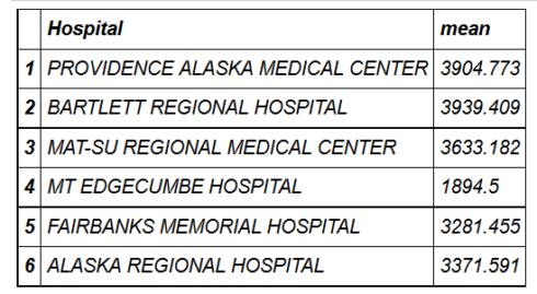
mygroup= group_by(hospital_spending,Hospital)
from_dplyr = summarize(mygroup,mean=mean(Avg.Spending.Per.Episode..Hospital.))
from_data_table=hospital_spending_DT[,.(mean=mean(Avg.Spending.Per.Episode..Hospital.)), by=.(Hospital)]
compare(from_dplyr,from_data_table, allowAll=TRUE)

TRUE
  sorted
  renamed rows
  dropped row names
  dropped attributes

We can also provide more than one grouping condition.

head(hospital_spending_DT[,.(mean=mean(Avg.Spending.Per.Episode..Hospital.)),
                          by=.(Hospital,State)])

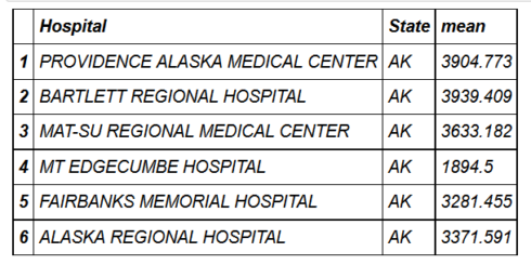
mygroup= group_by(hospital_spending,Hospital,State)
from_dplyr = summarize(mygroup,mean=mean(Avg.Spending.Per.Episode..Hospital.))
from_data_table=hospital_spending_DT[,.(mean=mean(Avg.Spending.Per.Episode..Hospital.)), by=.(Hospital,State)]
compare(from_dplyr,from_data_table, allowAll=TRUE)
TRUE
  sorted
  renamed rows
  dropped row names
  dropped attributes

Chaining

With both dplyr and data.table, we can chain functions in succession. In dplyr, we use pipes from the magrittr package with %>% which is really cool. %>% takes the output from one function and feeds it to the first argument of the next function. In data.table, we can use %>% or [ for chaining.

from_dplyr=hospital_spending%>%group_by(Hospital,State)%>%summarize(mean=mean(Avg.Spending.Per.Episode..Hospital.))
from_data_table=hospital_spending_DT[,.(mean=mean(Avg.Spending.Per.Episode..Hospital.)), by=.(Hospital,State)]
compare(from_dplyr,from_data_table, allowAll=TRUE)
TRUE
  sorted
  renamed rows
  dropped row names
  dropped attributes

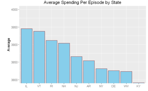
hospital_spending%>%group_by(State)%>%summarize(mean=mean(Avg.Spending.Per.Episode..Hospital.))%>%
arrange(desc(mean))%>%head(10)%>%
        mutate(State = factor(State,levels = State[order(mean,decreasing =TRUE)]))%>%
          ggplot(aes(x=State,y=mean))+geom_bar(stat='identity',color='darkred',fill='skyblue')+
          xlab("")+ggtitle('Average Spending Per Episode by State')+
          ylab('Average')+ coord_cartesian(ylim = c(3800, 4000))

hospital_spending_DT[,.(mean=mean(Avg.Spending.Per.Episode..Hospital.)),
                                     by=.(State)][order(-mean)][1:10]%>%
            mutate(State = factor(State,levels = State[order(mean,decreasing =TRUE)]))%>%
           ggplot(aes(x=State,y=mean))+geom_bar(stat='identity',color='darkred',fill='skyblue')+
          xlab("")+ggtitle('Average Spending Per Episode by State')+
          ylab('Average')+ coord_cartesian(ylim = c(3800, 4000))

Summary

In this blog post, we saw how we can perform the same tasks using data.tableand dplyr packages. Both packages have their strengths. While dplyr is more elegant and resembles natural language, data.table is succinct and we can do a lot with data.table in just a single line. Further, data.table is, in some cases, faster and it may be a go-to package when performance and memory are the constraints.

You can get the code for this blog post at my GitHub account.

This is enough for this post. If you have any questions or feedback, feel free to leave a comment.

转自：http://datascienceplus.com/best-packages-for-data-manipulation-in-r/