Chapter 4 深入理解Caffe MNIST DEMO中的LeNet网络模型
明代思想家王阳明提出了“知行合一”,谓认识事物的道理与在现实中运用此道理,是密不可分的一回事。我以为这样的中国哲学话语,对于学习者来说,极具启发意义,要细细体会。中华文明源远流长,很多做人做事的道理,孕育其中,需用心体会,并学以致用。
以“知”促“行”、以“行”促“知”、知行合一。——The unity of Inner knowledge and action.
在chapter 3 中提供了一个很好的实践样例,这个样例在windows下运行了Caffe源代码的MNIST Demo。本章将以该实践为基础来深入理解LeNet网络模型。
1. 初见LeNet原始模型
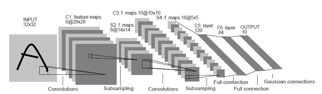
Fig.1. Architecture of original LeNet-5.
图片来源: Lecun, et al., Gradient-based learning applied to document recognition, P IEEE, vol. 86, no. 11, 1998, pp. 2278-2324.
在这篇图片的论文中,详细描述了LeNet-5的结构。
这里不对LeNet-5原始模型进行讨论。可以参考这些资料:
http://blog.csdn.net/qiaofangjie/article/details/16826849
http://blog.csdn.net/xuanyuansen/article/details/41800721
2. Caffe LeNet的网络结构
他山之石,可以攻玉。本来是准备画出Caffe LeNet的图的,但发现已经有人做了,并且画的很好,就直接拿过来辅助理解了。
第3部分图片来源:http://www.2cto.com/kf/201606/518254.html
先从整体上感知Caffe LeNet的拓扑图,由于Caffe中定义网络的结构采用的是bottom&top这种上下结构,所以这里的图也采用这种方式展现出来,更加方便理解。
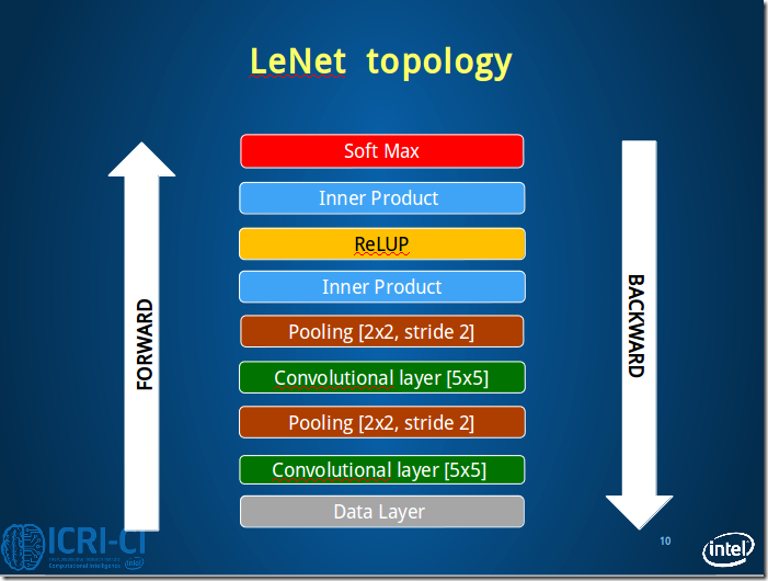
Fig.2. Architecture of caffe LeNet.
From bottom to top: Data Layer, conv1, pool1, conv2, pool2, ip1, relu1, ip2, [accuracy]loss.
本节接下来将按照这个顺序依次理解Caffe LeNet的网络结构。
3. 逐层理解Caffe LeNet
本节将采用定义与图解想结合的方式逐层理解Caffe LeNet的结构。
3.1 Data Layer
#==============定义TRAIN的数据层============================================
layer {
name: "mnist" #定义该层的名字
type: "Data" #该层的类型是数据
top: "data" #该层生成一个data blob
top: "label" #该层生成一个label blob
include {
phase: TRAIN #说明该层只在TRAIN阶段使用
}
transform_param {
scale: 0.00390625 #数据归一化系数,1/256,归一到[0,1)
}
data_param {
source: "E:/MyCode/DL/caffe-master/examples/mnist/mnist_train_lmdb" #训练数据的路径
batch_size: 64 #批量处理的大小
backend: LMDB
}
}
#==============定义TEST的数据层============================================
layer {
name: "mnist"
type: "Data"
top: "data"
top: "label"
include {
phase: TEST #说明该层只在TEST阶段使用
}
transform_param {
scale: 0.00390625
}
data_param {
source: "E:/MyCode/DL/caffe-master/examples/mnist/mnist_test_lmdb" #测试数据的路径
batch_size: 100
backend: LMDB
}
}
.csharpcode, .csharpcode pre
{
font-size: small;
color: black;
font-family: consolas, "Courier New", courier, monospace;
background-color: #ffffff;
/*white-space: pre;*/
}
.csharpcode pre { margin: 0em; }
.csharpcode .rem { color: #008000; }
.csharpcode .kwrd { color: #0000ff; }
.csharpcode .str { color: #006080; }
.csharpcode .op { color: #0000c0; }
.csharpcode .preproc { color: #cc6633; }
.csharpcode .asp { background-color: #ffff00; }
.csharpcode .html { color: #800000; }
.csharpcode .attr { color: #ff0000; }
.csharpcode .alt
{
background-color: #f4f4f4;
width: 100%;
margin: 0em;
}
.csharpcode .lnum { color: #606060; }
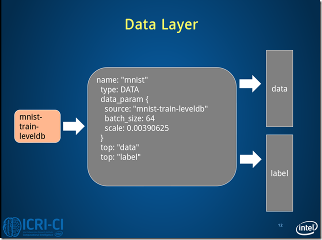
Fig.3. Architecture of data layer.
Fig.3 是train情况下,数据层读取lmdb数据,每次读取64条数据,即N=64。
Caffe中采用4D表示,N*C*H*W(Num*Channels*Height*Width)。
3.2 Conv1 Layer
#==============定义卷积层1=============================
layer {
name: "conv1" #该层的名字conv1,即卷积层1
type: "Convolution" #该层的类型是卷积层
bottom: "data" #该层使用的数据是由数据层提供的data blob
top: "conv1" #该层生成的数据是conv1
param {
lr_mult: 1 #weight learning rate(简写为lr)权值的学习率,1表示该值是lenet_solver.prototxt中base_lr: 0.01的1倍
}
param {
lr_mult: 2 #bias learning rate偏移值的学习率,2表示该值是lenet_solver.prototxt中base_lr: 0.01的2倍
}
convolution_param {
num_output: 20 #产生20个输出通道
kernel_size: 5 #卷积核的大小为5*5
stride: 1 #卷积核移动的步幅为1
weight_filler {
type: "xavier" #xavier算法,根据输入和输出的神经元的个数自动初始化权值比例
}
bias_filler {
type: "constant" #将偏移值初始化为“稳定”状态,即设为默认值0
}
}
}
.csharpcode, .csharpcode pre
{
font-size: small;
color: black;
font-family: consolas, "Courier New", courier, monospace;
background-color: #ffffff;
/*white-space: pre;*/
}
.csharpcode pre { margin: 0em; }
.csharpcode .rem { color: #008000; }
.csharpcode .kwrd { color: #0000ff; }
.csharpcode .str { color: #006080; }
.csharpcode .op { color: #0000c0; }
.csharpcode .preproc { color: #cc6633; }
.csharpcode .asp { background-color: #ffff00; }
.csharpcode .html { color: #800000; }
.csharpcode .attr { color: #ff0000; }
.csharpcode .alt
{
background-color: #f4f4f4;
width: 100%;
margin: 0em;
}
.csharpcode .lnum { color: #606060; }
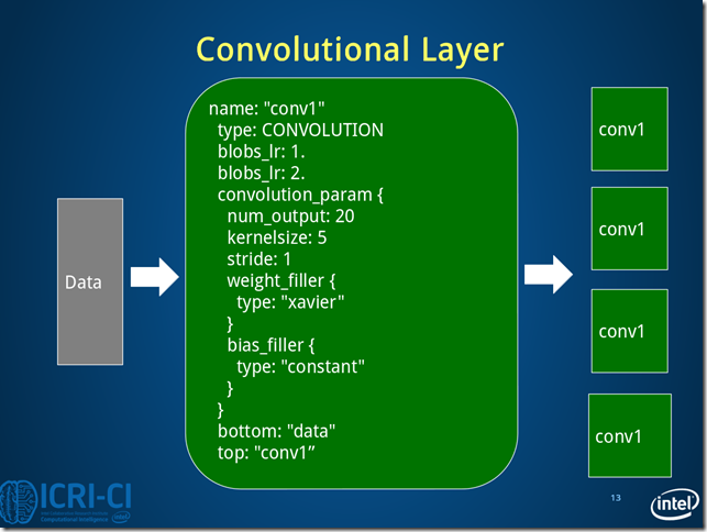
Fig.4. Architecture of conv1 layer.
conv1的数据变化的情况:batch_size*1*28*28->batch_size*20*24*24
3.3 Pool1 Layer
#==============定义池化层1=============================
layer {
name: "pool1"
type: "Pooling"
bottom: "conv1" #该层使用的数据是由conv1层提供的conv1
top: "pool1" #该层生成的数据是pool1
pooling_param {
pool: MAX #采用最大值池化
kernel_size: 2 #池化核大小为2*2
stride: 2 #池化核移动的步幅为2,即非重叠移动
}
}
.csharpcode, .csharpcode pre
{
font-size: small;
color: black;
font-family: consolas, "Courier New", courier, monospace;
background-color: #ffffff;
/*white-space: pre;*/
}
.csharpcode pre { margin: 0em; }
.csharpcode .rem { color: #008000; }
.csharpcode .kwrd { color: #0000ff; }
.csharpcode .str { color: #006080; }
.csharpcode .op { color: #0000c0; }
.csharpcode .preproc { color: #cc6633; }
.csharpcode .asp { background-color: #ffff00; }
.csharpcode .html { color: #800000; }
.csharpcode .attr { color: #ff0000; }
.csharpcode .alt
{
background-color: #f4f4f4;
width: 100%;
margin: 0em;
}
.csharpcode .lnum { color: #606060; }
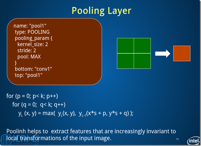
Fig.5. Architecture of pool1 layer.
池化层1过程数据变化:batch_size*20*24*24->batch_size*20*12*12
3.4 Conv2 Layer
#==============定义卷积层2=============================
layer {
name: "conv2"
type: "Convolution"
bottom: "pool1"
top: "conv2"
param {
lr_mult: 1
}
param {
lr_mult: 2
}
convolution_param {
num_output: 50
kernel_size: 5
stride: 1
weight_filler {
type: "xavier"
}
bias_filler {
type: "constant"
}
}
}
.csharpcode, .csharpcode pre
{
font-size: small;
color: black;
font-family: consolas, "Courier New", courier, monospace;
background-color: #ffffff;
/*white-space: pre;*/
}
.csharpcode pre { margin: 0em; }
.csharpcode .rem { color: #008000; }
.csharpcode .kwrd { color: #0000ff; }
.csharpcode .str { color: #006080; }
.csharpcode .op { color: #0000c0; }
.csharpcode .preproc { color: #cc6633; }
.csharpcode .asp { background-color: #ffff00; }
.csharpcode .html { color: #800000; }
.csharpcode .attr { color: #ff0000; }
.csharpcode .alt
{
background-color: #f4f4f4;
width: 100%;
margin: 0em;
}
.csharpcode .lnum { color: #606060; }
conv2层的图与Fig.4 类似,卷积层2过程数据变化:batch_size*20*12*12->batch_size*50*8*8。
3.5 Pool2 Layer
#==============定义池化层2=============================
layer {
name: "pool2"
type: "Pooling"
bottom: "conv2"
top: "pool2"
pooling_param {
pool: MAX
kernel_size: 2
stride: 2
}
}
.csharpcode, .csharpcode pre
{
font-size: small;
color: black;
font-family: consolas, "Courier New", courier, monospace;
background-color: #ffffff;
/*white-space: pre;*/
}
.csharpcode pre { margin: 0em; }
.csharpcode .rem { color: #008000; }
.csharpcode .kwrd { color: #0000ff; }
.csharpcode .str { color: #006080; }
.csharpcode .op { color: #0000c0; }
.csharpcode .preproc { color: #cc6633; }
.csharpcode .asp { background-color: #ffff00; }
.csharpcode .html { color: #800000; }
.csharpcode .attr { color: #ff0000; }
.csharpcode .alt
{
background-color: #f4f4f4;
width: 100%;
margin: 0em;
}
.csharpcode .lnum { color: #606060; }
pool2层图与Fig.5类似,池化层2过程数据变化:batch_size*50*8*8->batch_size*50*4*4。
3.6 Ip1 Layer
#==============定义全连接层1=============================
layer {
name: "ip1"
type: "InnerProduct" #该层的类型为全连接层
bottom: "pool2"
top: "ip1"
param {
lr_mult: 1
}
param {
lr_mult: 2
}
inner_product_param {
num_output: 500 #有500个输出通道
weight_filler {
type: "xavier"
}
bias_filler {
type: "constant"
}
}
}
.csharpcode, .csharpcode pre
{
font-size: small;
color: black;
font-family: consolas, "Courier New", courier, monospace;
background-color: #ffffff;
/*white-space: pre;*/
}
.csharpcode pre { margin: 0em; }
.csharpcode .rem { color: #008000; }
.csharpcode .kwrd { color: #0000ff; }
.csharpcode .str { color: #006080; }
.csharpcode .op { color: #0000c0; }
.csharpcode .preproc { color: #cc6633; }
.csharpcode .asp { background-color: #ffff00; }
.csharpcode .html { color: #800000; }
.csharpcode .attr { color: #ff0000; }
.csharpcode .alt
{
background-color: #f4f4f4;
width: 100%;
margin: 0em;
}
.csharpcode .lnum { color: #606060; }
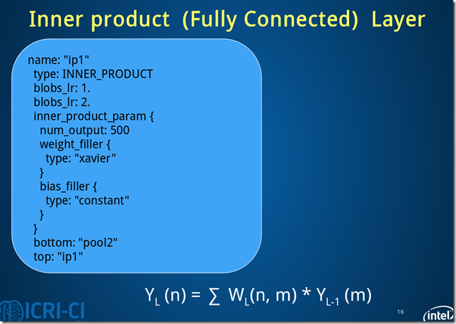
Fig.6. Architecture of ip11 layer.
ip1过程数据变化:batch_size*50*4*4->batch_size*500*1*1。
此处的全连接是将C*H*W转换成1D feature vector,即800->500.
3.7 Relu1 Layer
#==============定义ReLU1层=============================
layer {
name: "relu1"
type: "ReLU"
bottom: "ip1"
top: "ip1"
}

.csharpcode, .csharpcode pre
{
font-size: small;
color: black;
font-family: consolas, "Courier New", courier, monospace;
background-color: #ffffff;
/*white-space: pre;*/
}
.csharpcode pre { margin: 0em; }
.csharpcode .rem { color: #008000; }
.csharpcode .kwrd { color: #0000ff; }
.csharpcode .str { color: #006080; }
.csharpcode .op { color: #0000c0; }
.csharpcode .preproc { color: #cc6633; }
.csharpcode .asp { background-color: #ffff00; }
.csharpcode .html { color: #800000; }
.csharpcode .attr { color: #ff0000; }
.csharpcode .alt
{
background-color: #f4f4f4;
width: 100%;
margin: 0em;
}
.csharpcode .lnum { color: #606060; }
ReLU1层过程数据变化:batch_size*500*1*1->batch_size*500*1*1
3.8 Ip2 Layer
#==============定义全连接层2============================
layer {
name: "ip2"
type: "InnerProduct"
bottom: "ip1"
top: "ip2"
param {
lr_mult: 1
}
param {
lr_mult: 2
}
inner_product_param {
num_output: 10 #10个输出数据,对应0-9十个数字
weight_filler {
type: "xavier"
}
bias_filler {
type: "constant"
}
}
}
.csharpcode, .csharpcode pre
{
font-size: small;
color: black;
font-family: consolas, "Courier New", courier, monospace;
background-color: #ffffff;
/*white-space: pre;*/
}
.csharpcode pre { margin: 0em; }
.csharpcode .rem { color: #008000; }
.csharpcode .kwrd { color: #0000ff; }
.csharpcode .str { color: #006080; }
.csharpcode .op { color: #0000c0; }
.csharpcode .preproc { color: #cc6633; }
.csharpcode .asp { background-color: #ffff00; }
.csharpcode .html { color: #800000; }
.csharpcode .attr { color: #ff0000; }
.csharpcode .alt
{
background-color: #f4f4f4;
width: 100%;
margin: 0em;
}
.csharpcode .lnum { color: #606060; }
ip2过程数据变化:batch_size*500*1*1->batch_size*10*1*1
3.9 Loss Layer
#==============定义损失函数层============================
layer {
name: "loss"
type: "SoftmaxWithLoss"
bottom: "ip2"
bottom: "label"
top: "loss"
}
.csharpcode, .csharpcode pre
{
font-size: small;
color: black;
font-family: consolas, "Courier New", courier, monospace;
background-color: #ffffff;
/*white-space: pre;*/
}
.csharpcode pre { margin: 0em; }
.csharpcode .rem { color: #008000; }
.csharpcode .kwrd { color: #0000ff; }
.csharpcode .str { color: #006080; }
.csharpcode .op { color: #0000c0; }
.csharpcode .preproc { color: #cc6633; }
.csharpcode .asp { background-color: #ffff00; }
.csharpcode .html { color: #800000; }
.csharpcode .attr { color: #ff0000; }
.csharpcode .alt
{
background-color: #f4f4f4;
width: 100%;
margin: 0em;
}
.csharpcode .lnum { color: #606060; }
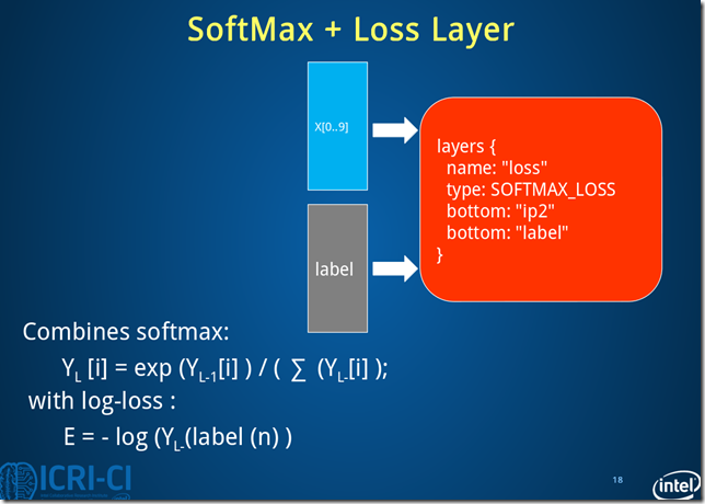
Fig.8. Architecture of loss layer.
损失层过程数据变化:batch_size*10*1*1->batch_size*10*1*1
note:注意到caffe LeNet中有一个accuracy layer的定义,这是输出测试结果的层。
4. Caffe LeNet的完整定义
name: "LeNet" #定义网络的名字
#==============定义TRAIN的数据层============================================
layer {
name: "mnist" #定义该层的名字
type: "Data" #该层的类型是数据
top: "data" #该层生成一个data blob
top: "label" #该层生成一个label blob
include {
phase: TRAIN #说明该层只在TRAIN阶段使用
}
transform_param {
scale: 0.00390625 #数据归一化系数,1/256,归一到[0,1)
}
data_param {
source: "E:/MyCode/DL/caffe-master/examples/mnist/mnist_train_lmdb" #训练数据的路径
batch_size: 64 #批量处理的大小
backend: LMDB
}
}
#==============定义TEST的数据层============================================
layer {
name: "mnist"
type: "Data"
top: "data"
top: "label"
include {
phase: TEST #说明该层只在TEST阶段使用
}
transform_param {
scale: 0.00390625
}
data_param {
source: "E:/MyCode/DL/caffe-master/examples/mnist/mnist_test_lmdb" #测试数据的路径
batch_size: 100
backend: LMDB
}
}
#==============定义卷积层1=============================
layer {
name: "conv1" #该层的名字conv1,即卷积层1
type: "Convolution" #该层的类型是卷积层
bottom: "data" #该层使用的数据是由数据层提供的data blob
top: "conv1" #该层生成的数据是conv1
param {
lr_mult: 1 #weight learning rate(简写为lr)权值的学习率,1表示该值是lenet_solver.prototxt中base_lr: 0.01的1倍
}
param {
lr_mult: 2 #bias learning rate偏移值的学习率,2表示该值是lenet_solver.prototxt中base_lr: 0.01的2倍
}
convolution_param {
num_output: 20 #产生20个输出通道
kernel_size: 5 #卷积核的大小为5*5
stride: 1 #卷积核移动的步幅为1
weight_filler {
type: "xavier" #xavier算法,根据输入和输出的神经元的个数自动初始化权值比例
}
bias_filler {
type: "constant" #将偏移值初始化为“稳定”状态,即设为默认值0
}
}
}#卷积过程数据变化:batch_size*1*28*28->batch_size*20*24*24
#==============定义池化层1=============================
layer {
name: "pool1"
type: "Pooling"
bottom: "conv1" #该层使用的数据是由conv1层提供的conv1
top: "pool1" #该层生成的数据是pool1
pooling_param {
pool: MAX #采用最大值池化
kernel_size: 2 #池化核大小为2*2
stride: 2 #池化核移动的步幅为2,即非重叠移动
}
}#池化层1过程数据变化:batch_size*20*24*24->batch_size*20*12*12
#==============定义卷积层2=============================
layer {
name: "conv2"
type: "Convolution"
bottom: "pool1"
top: "conv2"
param {
lr_mult: 1
}
param {
lr_mult: 2
}
convolution_param {
num_output: 50
kernel_size: 5
stride: 1
weight_filler {
type: "xavier"
}
bias_filler {
type: "constant"
}
}
}#卷积层2过程数据变化:batch_size*20*12*12->batch_size*50*8*8
#==============定义池化层2=============================
layer {
name: "pool2"
type: "Pooling"
bottom: "conv2"
top: "pool2"
pooling_param {
pool: MAX
kernel_size: 2
stride: 2
}
}#池化层2过程数据变化:batch_size*50*8*8->batch_size*50*4*4
#==============定义全连接层1=============================
layer {
name: "ip1"
type: "InnerProduct" #该层的类型为全连接层
bottom: "pool2"
top: "ip1"
param {
lr_mult: 1
}
param {
lr_mult: 2
}
inner_product_param {
num_output: 500 #有500个输出通道
weight_filler {
type: "xavier"
}
bias_filler {
type: "constant"
}
}
}#全连接层1过程数据变化:batch_size*50*4*4->batch_size*500*1*1
#==============定义ReLU1层=============================
layer {
name: "relu1"
type: "ReLU"
bottom: "ip1"
top: "ip1"
}#ReLU1层过程数据变化:batch_size*500*1*1->batch_size*500*1*1
#==============定义全连接层2============================
layer {
name: "ip2"
type: "InnerProduct"
bottom: "ip1"
top: "ip2"
param {
lr_mult: 1
}
param {
lr_mult: 2
}
inner_product_param {
num_output: 10 #10个输出数据,对应0-9十个数字
weight_filler {
type: "xavier"
}
bias_filler {
type: "constant"
}
}
}#全连接层2过程数据变化:batch_size*500*1*1->batch_size*10*1*1
#==============定义显示准确率结果层============================
layer {
name: "accuracy"
type: "Accuracy"
bottom: "ip2"
bottom: "label"
top: "accuracy"
include {
phase: TEST
}
}
#==============定义损失函数层============================
layer {
name: "loss"
type: "SoftmaxWithLoss"
bottom: "ip2"
bottom: "label"
top: "loss"
}#损失层过程数据变化:batch_size*10*1*1->batch_size*10*1*1
.csharpcode, .csharpcode pre
{
font-size: small;
color: black;
font-family: consolas, "Courier New", courier, monospace;
background-color: #ffffff;
/*white-space: pre;*/
}
.csharpcode pre { margin: 0em; }
.csharpcode .rem { color: #008000; }
.csharpcode .kwrd { color: #0000ff; }
.csharpcode .str { color: #006080; }
.csharpcode .op { color: #0000c0; }
.csharpcode .preproc { color: #cc6633; }
.csharpcode .asp { background-color: #ffff00; }
.csharpcode .html { color: #800000; }
.csharpcode .attr { color: #ff0000; }
.csharpcode .alt
{
background-color: #f4f4f4;
width: 100%;
margin: 0em;
}
.csharpcode .lnum { color: #606060; }
Chapter 4 深入理解Caffe MNIST DEMO中的LeNet网络模型的更多相关文章
- Chapter 3 Start Caffe with MNIST Demo
先从一个具体的例子来开始Caffe,以MNIST手写数据为例. 1.下载数据 下载mnist到caffe-master\data\mnist文件夹. THE MNIST DATABASE:Yann L ...
- caffe实际运行中遇到的问题
https://blog.csdn.net/u010417185/article/details/52649178 1.均值计算是否需要统一图像的尺寸? 在图像计算均值时,应该先统一图像的尺寸,否则会 ...
- IM开发基础知识补课(四):正确理解HTTP短连接中的Cookie、Session和Token
本文引用了简书作者“骑小猪看流星”技术文章“Cookie.Session.Token那点事儿”的部分内容,感谢原作者. 1.前言 众所周之,IM是个典型的快速数据流交换系统,当今主流IM系统(尤其移动 ...
- caffe web demo运行+源码分析
caffe web demo学习 1.运行 安装好caffe后,进入/opt/caffe/examples/web_demo/的caffe web demo项目目录,查看一下app.py文件,这是一个 ...
- qt的demo中,经常可以看到emum
最近开始看QT的文档,发现了很多好东西,至少对于我来说 收获很多~~~ 当然很多东西自己还不能理解的很透彻,也是和朋友讨论以后才渐渐清晰的,可能对于QT中一些经典的用意我还是存在会有些认识上的偏差,欢 ...
- 理解与应用css中的display属性
理解与应用css中的display属性 display属性是我们在前端开发中常常使用的一个属性,其中,最常见的有: none block inline inline-block inherit 下面, ...
- 理解和使用 JavaScript 中的回调函数
理解和使用 JavaScript 中的回调函数 标签: 回调函数指针js 2014-11-25 01:20 11506人阅读 评论(4) 收藏 举报 分类: JavaScript(4) 目录( ...
- [转]理解与使用Javascript中的回调函数
在Javascript中,函数是第一类对象,这意味着函数可以像对象一样按照第一类管理被使用.既然函数实际上是对象:它们能被“存储”在变量中,能作为函数参数被传递,能在函数中被创建,能从函数中返回. 因 ...
- 【JavaScript】理解与使用Javascript中的回调函数
在Javascript中,函数是第一类对象,这意味着函数可以像对象一样按照第一类管理被使用.既然函数实际上是对象:它们能被“存储”在变量中,能作为函数参数被传递,能在函数中被创建,能从函数中返回. 因 ...
随机推荐
- Springboot+Thymeleaf框架的button错误
---恢复内容开始--- 在做公司项目时,遇到了一个Springboot+Thymeleaf框架问题: 使用框架写网站时,没有标明type类型的button默认成了‘submit’类型,每次点击按钮都 ...
- 【刷题】BZOJ 3591 最长上升子序列
Description 给出1~n的一个排列的一个最长上升子序列,求原排列可能的种类数. Input 第一行一个整数n. 第二行一个整数k,表示最长上升子序列的长度. 第三行k个整数,表示这个最长上升 ...
- 51nod 1494 选举拉票 | 线段树
51nod1494 选举拉票 题面 现在你要竞选一个县的县长.你去对每一个选民进行了调查.你已经知道每一个人要选的人是谁,以及要花多少钱才能让这个人选你.现在你想要花最少的钱使得你当上县长.你当选的条 ...
- 51nod 1295 XOR key | 可持久化Trie树
51nod 1295 XOR key 这也是很久以前就想做的一道板子题了--学了一点可持久化之后我终于会做这道题了! 给出一个长度为N的正整数数组A,再给出Q个查询,每个查询包括3个数,L, R, X ...
- Alpha 冲刺 —— 十分之九
队名 火箭少男100 组长博客 林燊大哥 作业博客 Alpha 冲鸭鸭鸭鸭鸭鸭鸭鸭鸭! 成员冲刺阶段情况 林燊(组长) 过去两天完成了哪些任务 协调各成员之间的工作 多次测试软件运行 学习OPENMP ...
- Web项目开发中用到的缓存技术
在WEB开发中用来应付高流量最有效的办法就是用缓存技术,能有效的提高服务器负载性能,用空间换取时间.缓存一般用来 存储频繁访问的数据 临时存储耗时的计算结果 内存缓存减少磁盘IO 使用缓存的2个主要原 ...
- 287find-the-duplicate-number
某视面试官问了一道这样的题,1到N(N为正整数)共N个正整数,其中有一个数重复一次覆盖了另外一个数,比如:9,3,7,5,1,8,2,4,5,那么其中5重复一次,相当于覆盖了6,那么,请找出这个重复的 ...
- 【Asp.net入门3-04】使用jQuery-使用jQuery事件
- Docker Swarm应用--lnmp部署WordPress
一.简介 目的:使用Docker Swarm 搭建lnmp来部署WordPress 使用Dockerfile构建nginx.php镜像 将构建的镜像上传docker私有仓库 使用volume做work ...
- linux命令总结之traceroute命令
通过traceroute我们可以知道信息从你的计算机到互联网另一端的主机是走的什么路径.当然每次数据包由某一同样的出发点(source)到达某一同样的目的地(destination)走的路径可能会不一 ...